Exploring data I

Lecture 4

John Zito

Duke University
STA 199 Spring 2025

2025-01-23

While you wait…

Prepare for today’s application exercise: ae-03-gerrymander-explore-I

Switch to your ae project in RStudio;
Make sure all of your changes up to this point are committed (ie there’s nothing left in your Git pane);
Click Pull to get today’s application exercise file: ae-03-gerrymander-explore-I.qmd.
Then push. So Render > Commit > Pull > Push.
Wait till the you’re prompted to work on the application exercise during class before editing the file.

AEs are due by the end of class

Successful completion means at least one commit + push by 2PM today

Exploratory data analysis

Packages

For the data: usdata

library(usdata)

For the analysis: tidyverse and ggthemes

library(tidyverse)
library(ggthemes)

Data: `gerrymander`

gerrymander

# A tibble: 435 × 12
   district last_name first_name party16 clinton16 trump16 dem16 state party18
   <chr>    <chr>     <chr>      <chr>       <dbl>   <dbl> <dbl> <chr> <chr>  
 1 AK-AL    Young     Don        R            37.6    52.8     0 AK    R      
 2 AL-01    Byrne     Bradley    R            34.1    63.5     0 AL    R      
 3 AL-02    Roby      Martha     R            33      64.9     0 AL    R      
 4 AL-03    Rogers    Mike D.    R            32.3    65.3     0 AL    R      
 5 AL-04    Aderholt  Rob        R            17.4    80.4     0 AL    R      
 6 AL-05    Brooks    Mo         R            31.3    64.7     0 AL    R      
 7 AL-06    Palmer    Gary       R            26.1    70.8     0 AL    R      
 8 AL-07    Sewell    Terri      D            69.8    28.6     1 AL    D      
 9 AR-01    Crawford  Rick       R            30.2    65       0 AR    R      
10 AR-02    Hill      French     R            41.7    52.4     0 AR    R      
# ℹ 425 more rows
# ℹ 3 more variables: dem18 <dbl>, flip18 <dbl>, gerry <fct>

What is gerrymandering?

JZ’s tour of the USA

JZ’s tour of the USA

JZ’s tour of the USA

JZ’s tour of the USA

Data: `gerrymander`

What is a good first function to use to get to know a dataset?

glimpse(gerrymander)

Rows: 435
Columns: 12
$ district   <chr> "AK-AL", "AL-01", "AL-02", "AL-03", "AL-04", "AL-05", "AL-0…
$ last_name  <chr> "Young", "Byrne", "Roby", "Rogers", "Aderholt", "Brooks", "…
$ first_name <chr> "Don", "Bradley", "Martha", "Mike D.", "Rob", "Mo", "Gary",…
$ party16    <chr> "R", "R", "R", "R", "R", "R", "R", "D", "R", "R", "R", "R",…
$ clinton16  <dbl> 37.6, 34.1, 33.0, 32.3, 17.4, 31.3, 26.1, 69.8, 30.2, 41.7,…
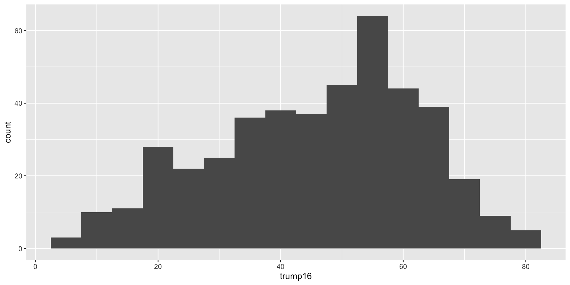
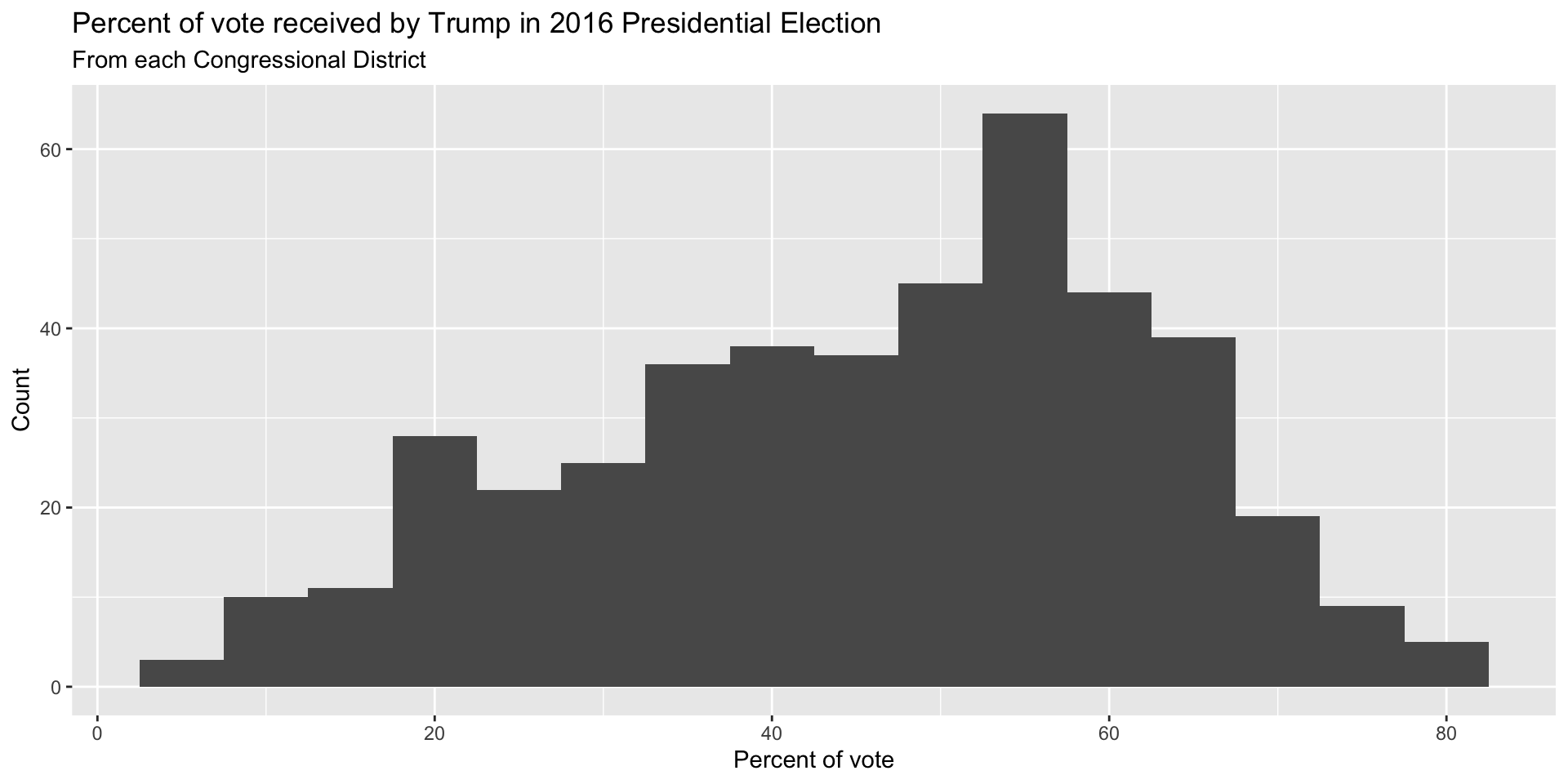
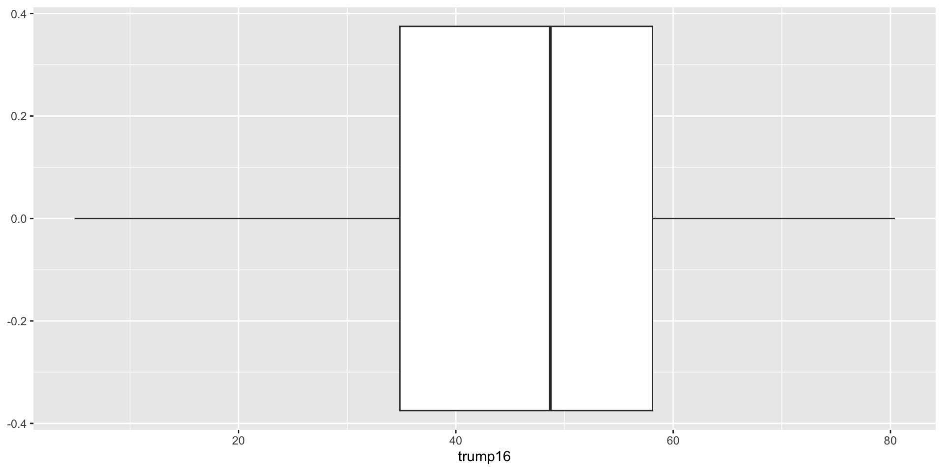
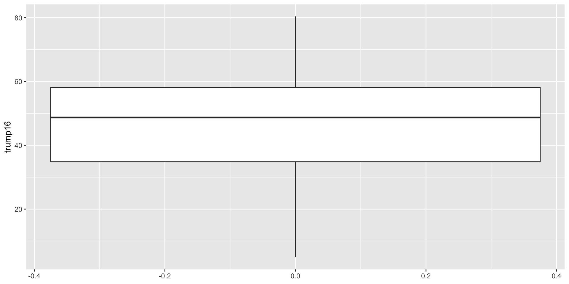
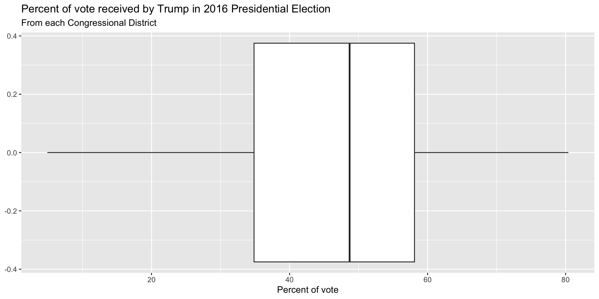
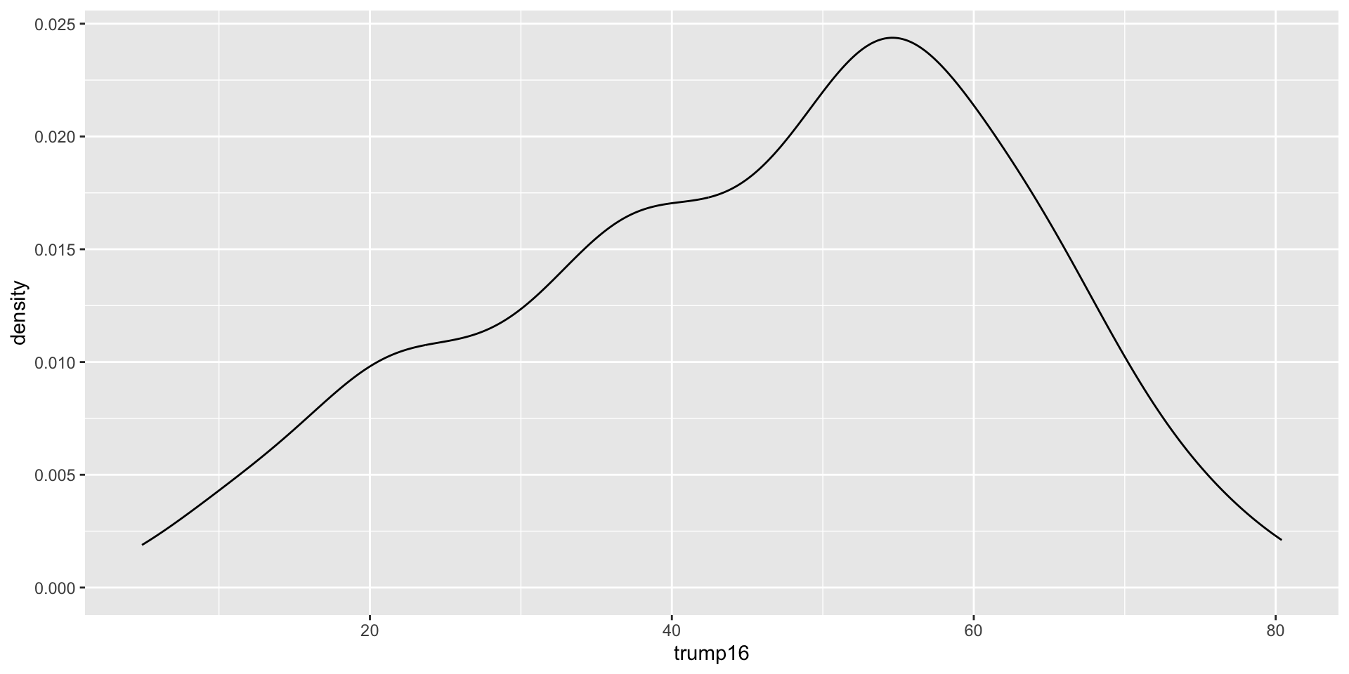
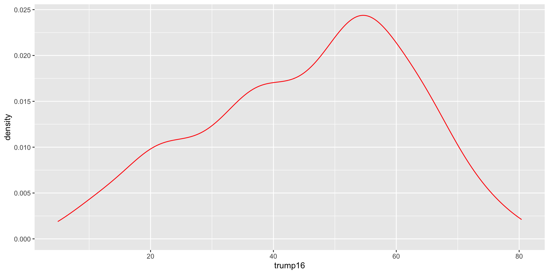
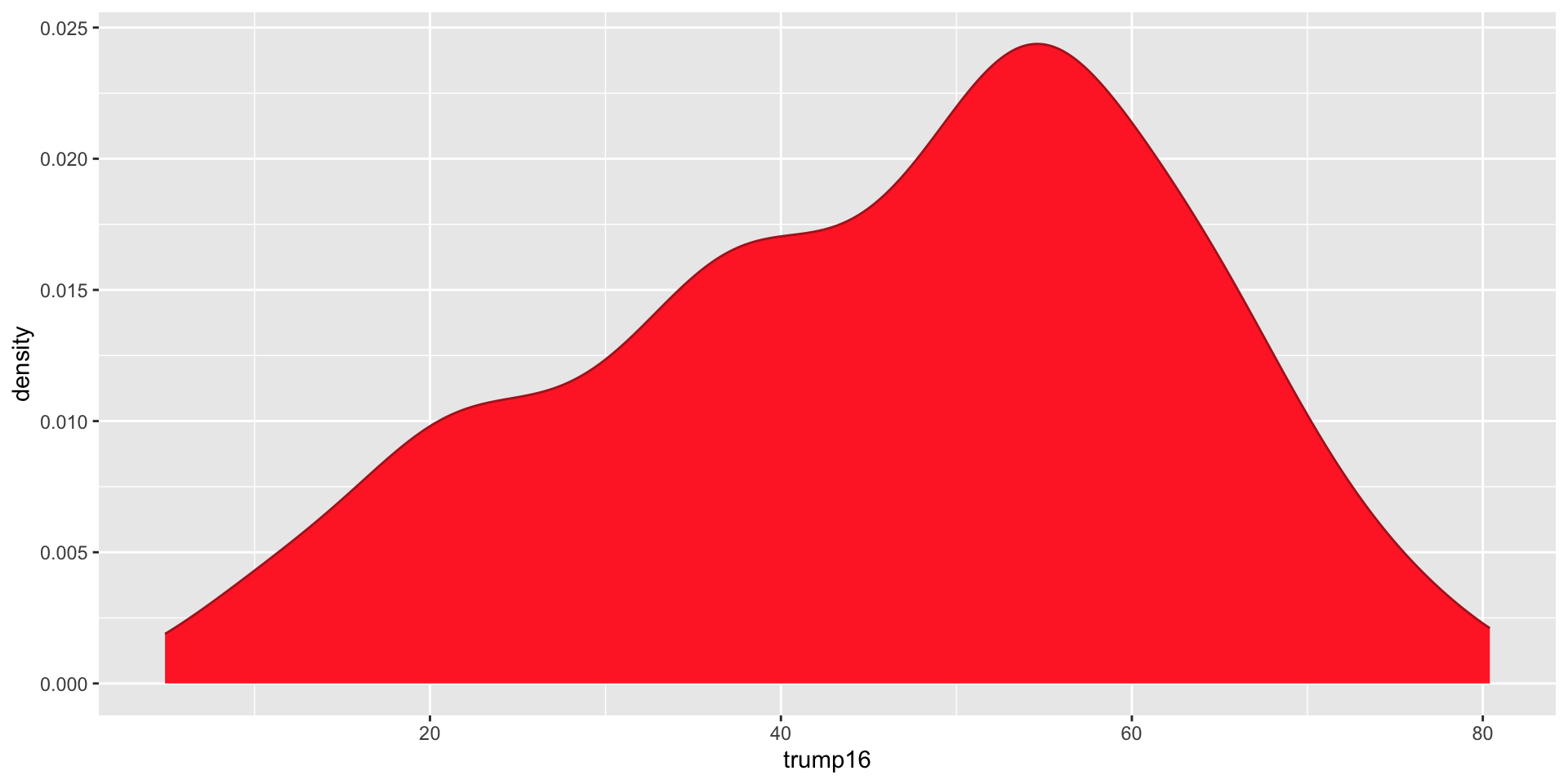
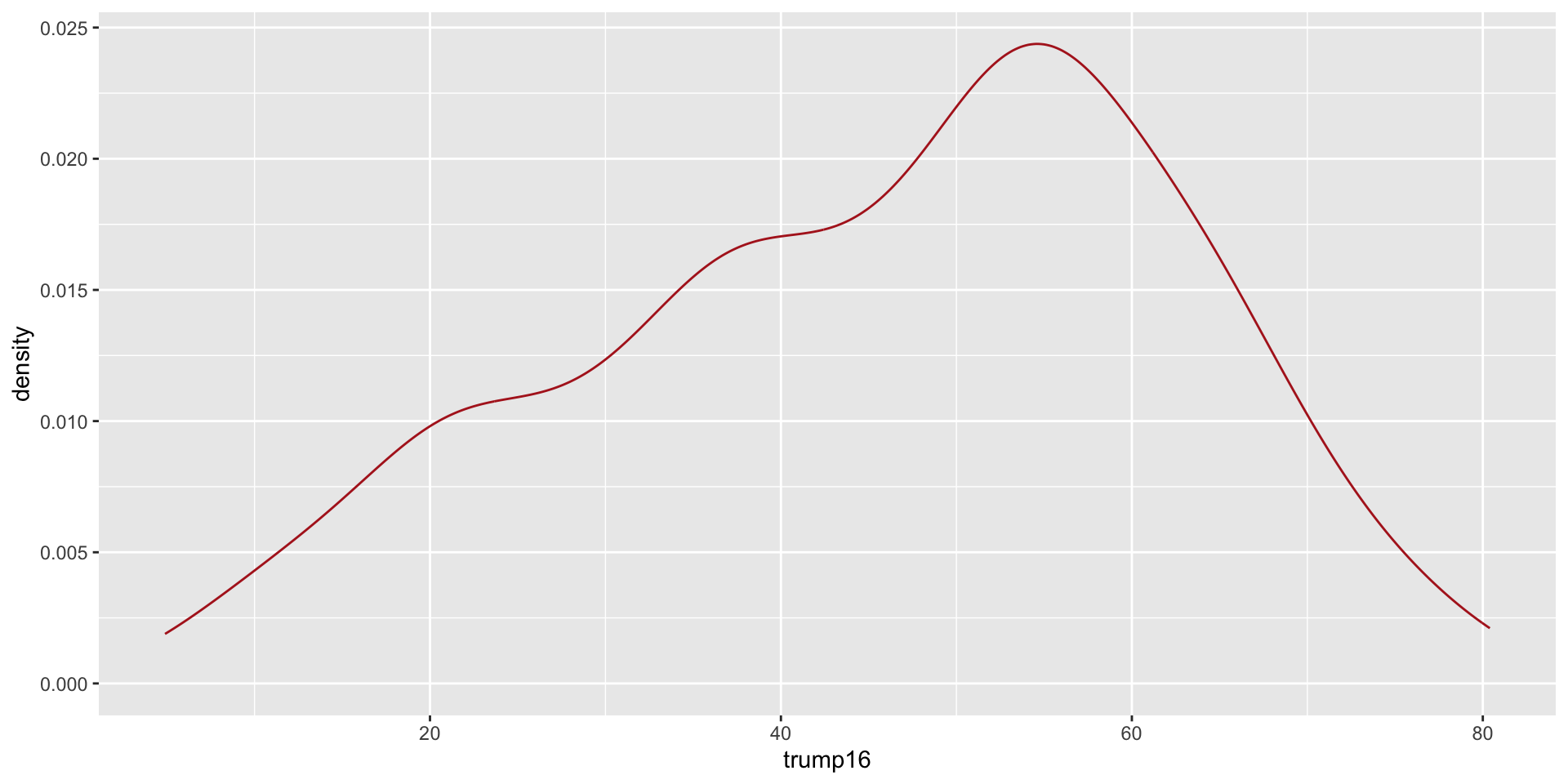
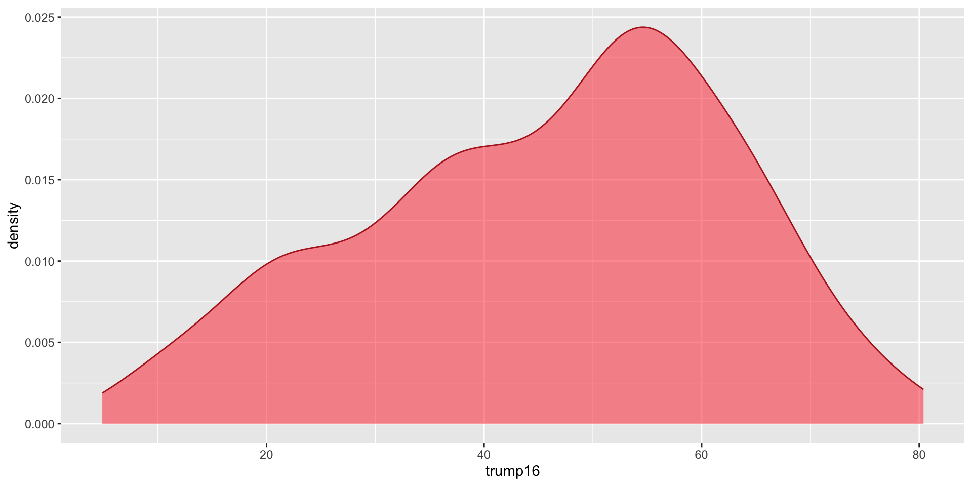
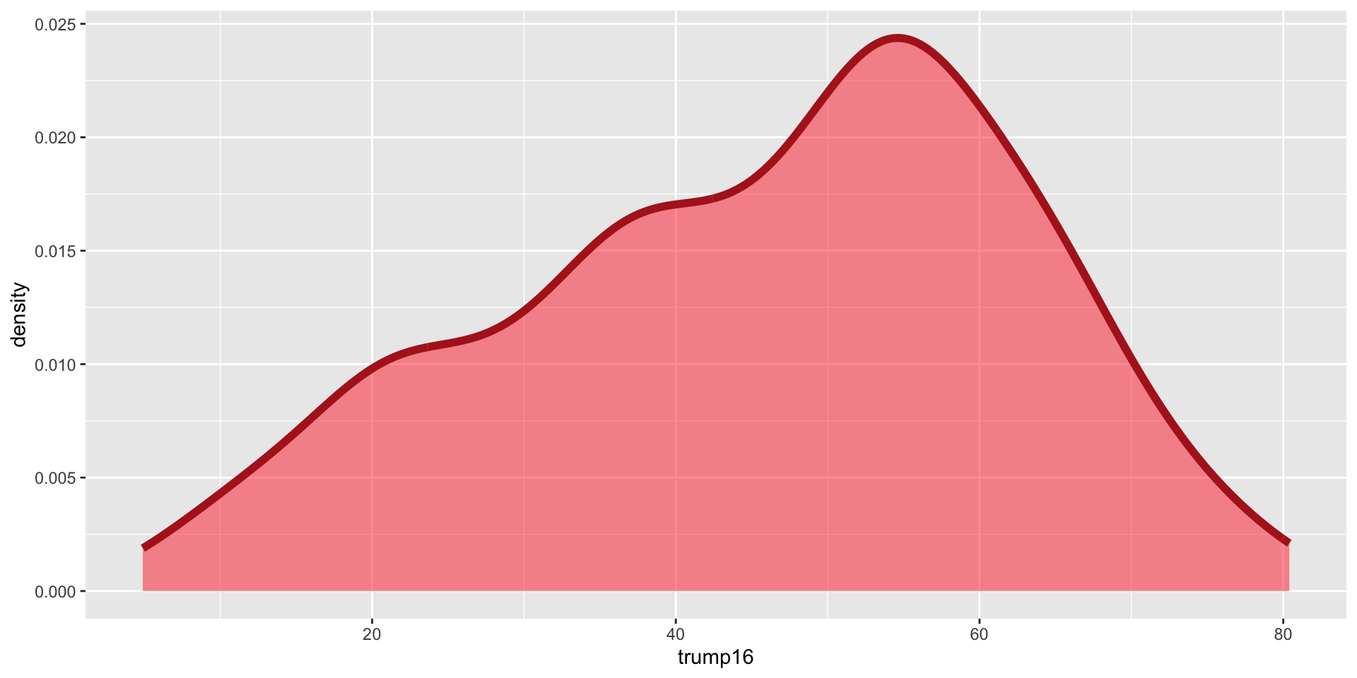
$ trump16    <dbl> 52.8, 63.5, 64.9, 65.3, 80.4, 64.7, 70.8, 28.6, 65.0, 52.4,…
$ dem16      <dbl> 0, 0, 0, 0, 0, 0, 0, 1, 0, 0, 0, 0, 1, 0, 1, 0, 0, 0, 1, 0,…
$ state      <chr> "AK", "AL", "AL", "AL", "AL", "AL", "AL", "AL", "AR", "AR",…
$ party18    <chr> "R", "R", "R", "R", "R", "R", "R", "D", "R", "R", "R", "R",…
$ dem18      <dbl> 0, 0, 0, 0, 0, 0, 0, 1, 0, 0, 0, 0, 1, 1, 1, 0, 0, 0, 1, 0,…
$ flip18     <dbl> 0, 0, 0, 0, 0, 0, 0, 0, 0, 0, 0, 0, 0, 1, 0, 0, 0, 0, 0, 0,…
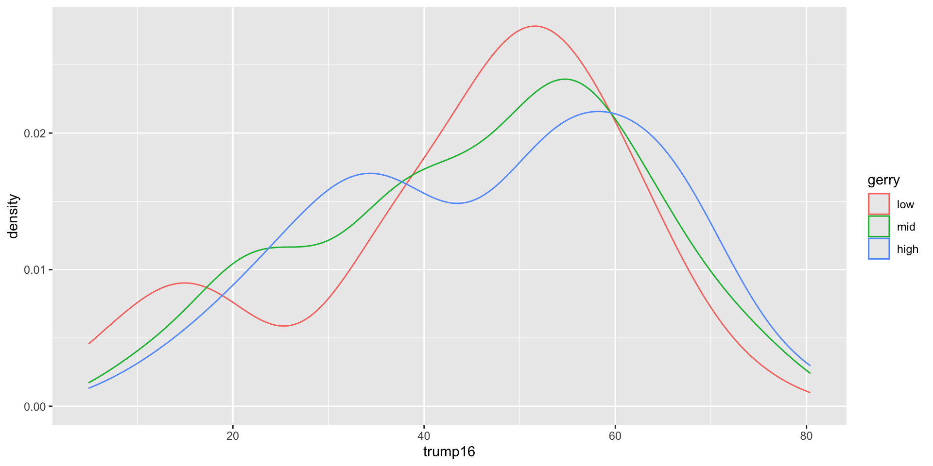
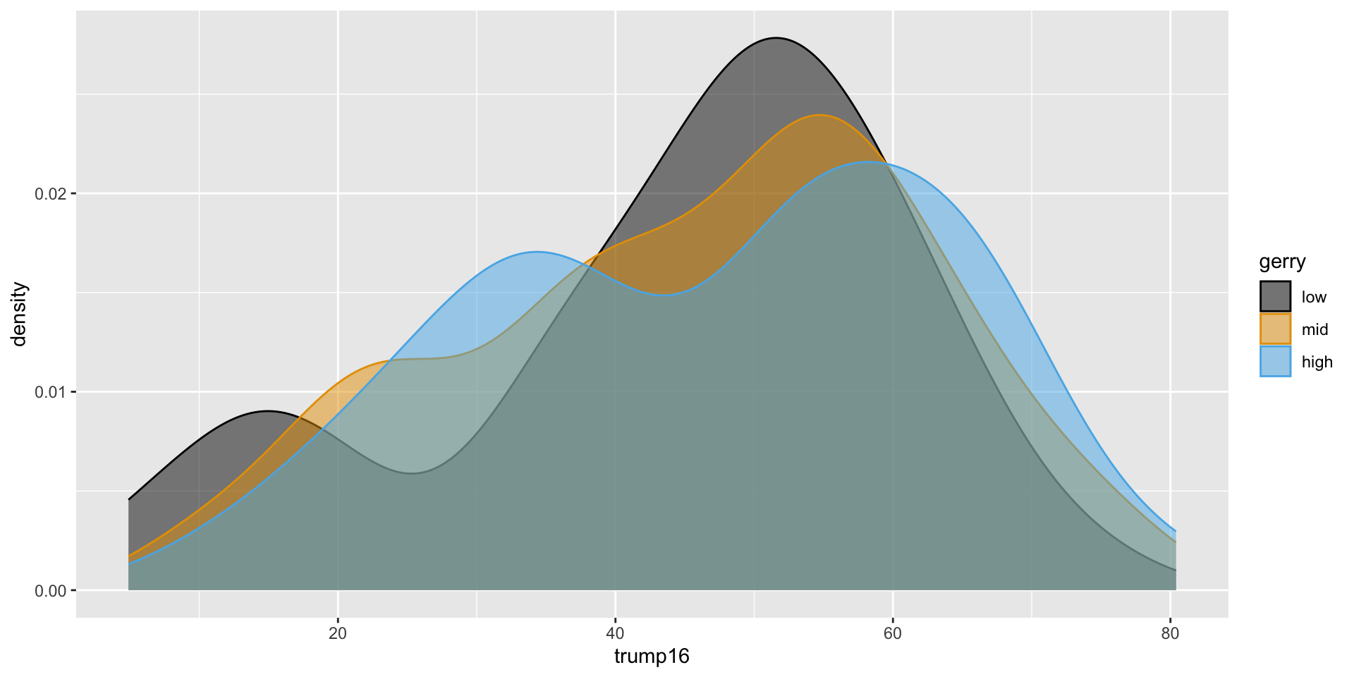
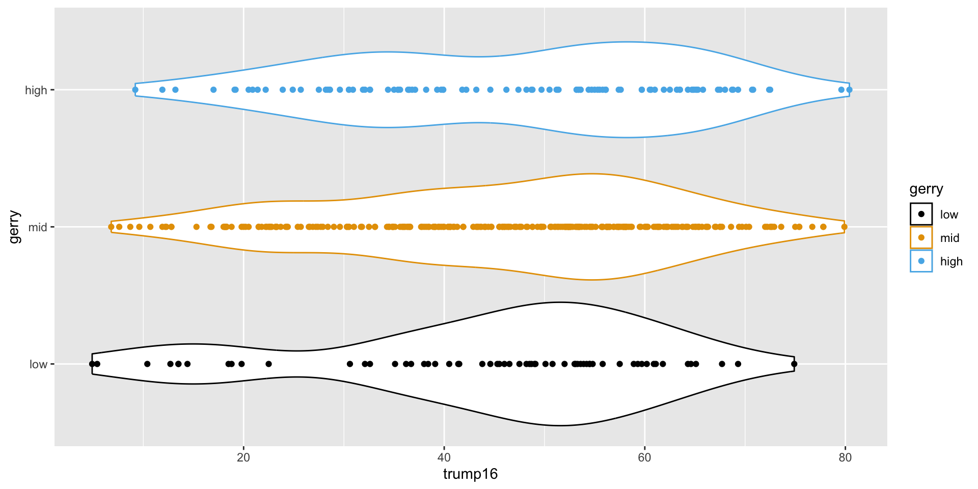
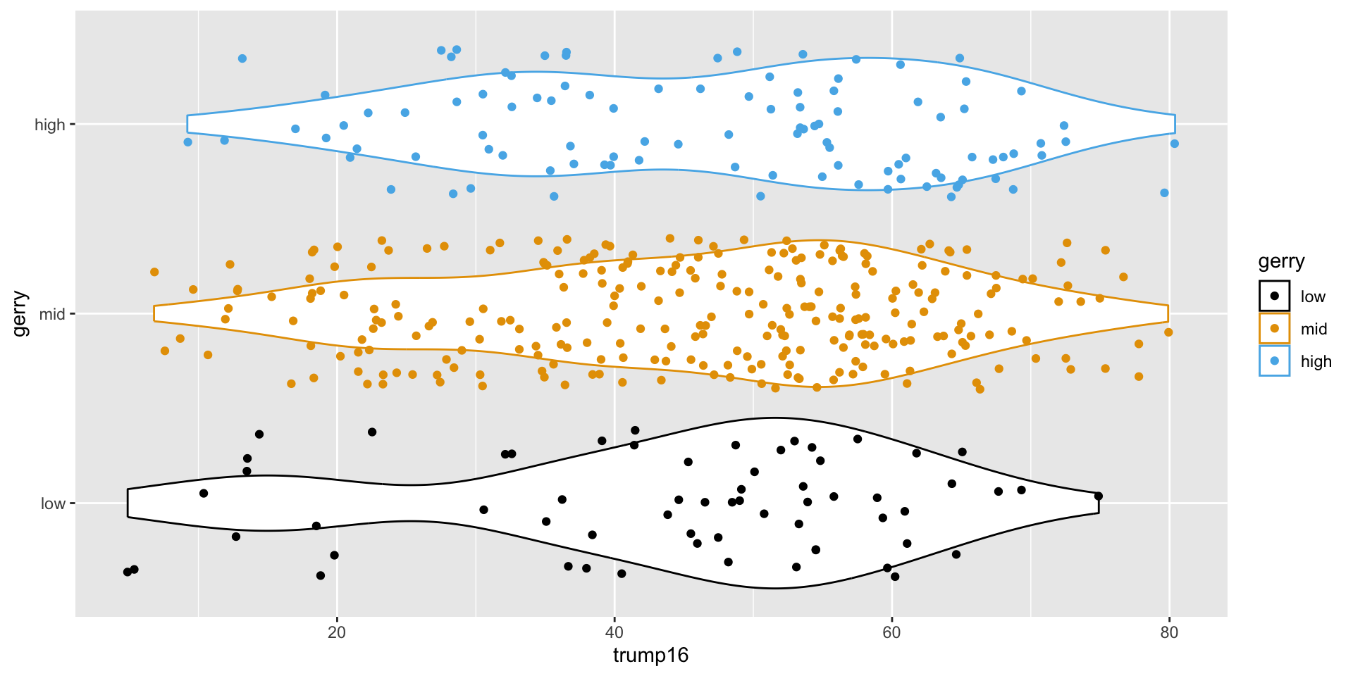
$ gerry      <fct> mid, high, high, high, high, high, high, high, mid, mid, mi…

Data: `gerrymander`

Rows: Congressional districts
Columns:
- Congressional district and state
- 2016 election: winning party, % for Clinton, % for Trump, whether a Democrat won the House election, name of election winner
- 2018 election: winning party, whether a Democrat won the 2018 House election
- Whether a Democrat flipped the seat in the 2018 election
- Prevalence of gerrymandering: low, mid, and high

Variable types

Variable	Type
`district`	categorical, ID
`last_name`	categorical, ID
`first_name`	categorical, ID
`party16`	categorical
`clinton16`	numerical, continuous
`trump16`	numerical, continuous

Variable	Type
`dem16`	categorical
`state`	categorical
`party18`	categorical
`dem18`	categorical
`flip18`	categorical
`gerry`	categorical, ordinal

Univariate analysis

Analyzing a single variable:

Numerical: histogram, box plot, density plot, etc.
Categorical: bar plot, pie chart, etc.

Histogram - Step 1

ggplot(gerrymander)

Histogram - Step 2

ggplot(gerrymander, aes(x = trump16))

Histogram - Step 3

ggplot(gerrymander, aes(x = trump16)) +
  geom_histogram()

Histogram - Step 4

ggplot(gerrymander, aes(x = trump16)) +
  geom_histogram(binwidth = 1)

Histogram - Step 4

ggplot(gerrymander, aes(x = trump16)) +
  geom_histogram(binwidth = 100)

Histogram - Step 4

ggplot(gerrymander, aes(x = trump16)) +
  geom_histogram(binwidth = 3)

Histogram - Step 4

ggplot(gerrymander, aes(x = trump16)) +
  geom_histogram(binwidth = 5)

Histogram - Step 5

ggplot(gerrymander, aes(x = trump16)) +
  geom_histogram(binwidth = 5) +
  labs(
    title = "Percent of vote received by Trump in 2016 Presidential Election",
    subtitle = "From each Congressional District",
    x = "Percent of vote",
    y = "Count"
  )

Box plot - Step 1

ggplot(gerrymander)

Box plot - Step 2

ggplot(gerrymander, aes(x = trump16))

Box plot - Step 3

ggplot(gerrymander, aes(x = trump16)) +
  geom_boxplot()

Box plot - Alternative Step 2 + 3

ggplot(gerrymander, aes(y = trump16)) +
  geom_boxplot()

Box plot - Step 4

ggplot(gerrymander, aes(x = trump16)) +
  geom_boxplot() +
  labs(
    title = "Percent of vote received by Trump in 2016 Presidential Election",
    subtitle = "From each Congressional District",
    x = "Percent of vote",
    y = NULL
  )

Density plot - Step 1

ggplot(gerrymander)

Density plot - Step 2

ggplot(gerrymander, aes(x = trump16))

Density plot - Step 3

ggplot(gerrymander, aes(x = trump16)) +
  geom_density()

Density plot - Step 4

ggplot(gerrymander, aes(x = trump16)) +
  geom_density(color = "red")

Density plot - Step 5

ggplot(gerrymander, aes(x = trump16)) +
  geom_density(color = "firebrick", fill = "firebrick1")

Density plot - Step 6

ggplot(gerrymander, aes(x = trump16)) +
  geom_density(color = "firebrick", fill = "firebrick1", alpha = 1)

Density plot - Step 6

ggplot(gerrymander, aes(x = trump16)) +
  geom_density(color = "firebrick", fill = "firebrick1", alpha = 0)

Density plot - Step 6

ggplot(gerrymander, aes(x = trump16)) +
  geom_density(color = "firebrick", fill = "firebrick1", alpha = 0.5)

Density plot - Step 7

ggplot(gerrymander, aes(x = trump16)) +
  geom_density(color = "firebrick", fill = "firebrick1", alpha = 0.5, linewidth = 2)

Density plot - Step 8

ggplot(gerrymander, aes(x = trump16)) +
  geom_density(color = "firebrick", fill = "firebrick1", alpha = 0.5, linewidth = 2) +
  labs(
    title = "Percent of vote received by Trump in 2016 Presidential Election",
    subtitle = "From each Congressional District",
    x = "Percent of vote",
    y = "Density"
  )

Summary statistics

gerrymander |>
  summarize(
    mean_trump_perc = mean(trump16),
    median_trump_perc = median(trump16),
    sd = sd(trump16),
    iqr = IQR(trump16),
    q25 = quantile(trump16, 0.25),
    q75 = quantile(trump16, 0.75)
  )

# A tibble: 1 × 6
  mean_trump_perc median_trump_perc    sd   iqr   q25   q75
            <dbl>             <dbl> <dbl> <dbl> <dbl> <dbl>
1            45.9              48.7  16.8  23.3  34.8  58.1

Distribution of votes for Trump in the 2016 election

Describe the distribution of percent of vote received by Trump in 2016 Presidential Election from Congressional Districts.

Shape: The distribution of votes for Trump in the 2016 election from Congressional Districts is unimodal and left-skewed.
Center: The percent of vote received by Trump in the 2016 Presidential Election from a typical Congressional Districts is 48.7%.
Spread: In the middle 50% of Congressional Districts, 34.8% to 58.1% of voters voted for Trump in the 2016 Presidential Election.
Unusual observations: -

Bivariate analysis

Analyzing the relationship between two variables:

Numerical + numerical: scatterplot
Numerical + categorical: side-by-side box plots, violin plots, etc.
Categorical + categorical: stacked bar plots
Using an aesthetic (e.g., fill, color, shape, etc.) or facets to represent the second variable in any plot

Side-by-side box plots

ggplot(
  gerrymander, 
  aes(
    x = trump16, 
    y = gerry
    )
  ) +
  geom_boxplot()

Summary statistics

gerrymander |>
  # do the following for each level of gerry
  summarize(
    min = min(trump16),
    q25 = quantile(trump16, 0.25),
    median = median(trump16),
    q75 = quantile(trump16, 0.75),
    max = max(trump16),
  )

# A tibble: 1 × 5
    min   q25 median   q75   max
  <dbl> <dbl>  <dbl> <dbl> <dbl>
1   4.9  34.8   48.7  58.1  80.4

Summary statistics

gerrymander |>
  filter(gerry == "low") |>
  summarize(
    min = min(trump16),
    q25 = quantile(trump16, 0.25),
    median = median(trump16),
    q75 = quantile(trump16, 0.75),
    max = max(trump16),
  )

# A tibble: 1 × 5
    min   q25 median   q75   max
  <dbl> <dbl>  <dbl> <dbl> <dbl>
1   4.9  36.3   48.4  54.7  74.9

Summary statistics

gerrymander |>
  filter(gerry == "mid") |>
  summarize(
    min = min(trump16),
    q25 = quantile(trump16, 0.25),
    median = median(trump16),
    q75 = quantile(trump16, 0.75),
    max = max(trump16),
  )

# A tibble: 1 × 5
    min   q25 median   q75   max
  <dbl> <dbl>  <dbl> <dbl> <dbl>
1   6.8  34.8   48.0  57.9  79.9

Summary statistics

gerrymander |>
  filter(gerry == "high") |>
  summarize(
    min = min(trump16),
    q25 = quantile(trump16, 0.25),
    median = median(trump16),
    q75 = quantile(trump16, 0.75),
    max = max(trump16),
  )

# A tibble: 1 × 5
    min   q25 median   q75   max
  <dbl> <dbl>  <dbl> <dbl> <dbl>
1   9.2  33.5   50.5  60.8  80.4

Summary statistics

gerrymander |>
  group_by(gerry) |>
  summarize(
    min = min(trump16),
    q25 = quantile(trump16, 0.25),
    median = median(trump16),
    q75 = quantile(trump16, 0.75),
    max = max(trump16),
  )

# A tibble: 3 × 6
  gerry   min   q25 median   q75   max
  <fct> <dbl> <dbl>  <dbl> <dbl> <dbl>
1 low     4.9  36.3   48.4  54.7  74.9
2 mid     6.8  34.8   48.0  57.9  79.9
3 high    9.2  33.5   50.5  60.8  80.4

Density plots

ggplot(
  gerrymander, 
  aes(
    x = trump16, 
    color = gerry
    )
  ) +
  geom_density()

Filled density plots

ggplot(
  gerrymander, 
  aes(
    x = trump16, 
    color = gerry,
    fill = gerry
    )
  ) +
  geom_density()

Better filled density plots

ggplot(
  gerrymander, 
  aes(x = trump16, color = gerry, fill = gerry)
  ) +
  geom_density(alpha = 0.5)

Better colors

ggplot(
  gerrymander, 
  aes(x = trump16, color = gerry, fill = gerry)
  ) +
  geom_density(alpha = 0.5) +
  scale_color_colorblind() +
  scale_fill_colorblind()

Violin plots

ggplot(
  gerrymander, 
  aes(x = trump16, y = gerry, color = gerry)
  ) +
  geom_violin() +
  scale_color_colorblind() +
  scale_fill_colorblind()

Multiple geoms

ggplot(
  gerrymander, 
  aes(x = trump16, y = gerry, color = gerry)
  ) +
  geom_violin() +
  geom_point() +
  scale_color_colorblind() +
  scale_fill_colorblind()

Multiple geoms

ggplot(
  gerrymander, 
  aes(x = trump16, y = gerry, color = gerry)
  ) +
  geom_violin() +
  geom_jitter() +
  scale_color_colorblind() +
  scale_fill_colorblind()

Remove legend

ggplot(
  gerrymander, 
  aes(x = trump16, y = gerry, color = gerry)
  ) +
  geom_violin() +
  geom_jitter() +
  scale_color_colorblind() +
  scale_fill_colorblind() +
  theme(legend.position = "none")

Multivariate analysis

Analyzing the relationship between multiple variables:

In general, one variable is identified as the outcome of interest
The remaining variables are predictors or explanatory variables
Plots for exploring multivariate relationships are the same as those for bivariate relationships, but conditional on one or more variables
- Conditioning can be done via faceting or aesthetic mappings (e.g., scatterplot of y vs. x1, colored by x2, faceted by x3)
Summary statistics for exploring multivariate relationships are the same as those for bivariate relationships, but conditional on one or more variables
- Conditioning can be done via grouping (e.g., correlation between y and x1, grouped by levels of x2 and x3)

Application exercise

ae-03-gerrymander-explore-I

Go to your ae project in RStudio.
If you haven’t yet done so, make sure all of your changes up to this point are committed and pushed, i.e., there’s nothing left in your Git pane.
If you haven’t yet done so, click Pull to get today’s application exercise file: ae-03-gerrymander-explore-I.qmd.
Work through the application exercise in class, and render, commit, and push your edits by the end of class.

Exploring data I

While you wait…

Exploratory data analysis

Packages

Data: gerrymander

What is gerrymandering?

JZ’s tour of the USA

JZ’s tour of the USA

JZ’s tour of the USA

JZ’s tour of the USA

Data: gerrymander

Data: gerrymander

Variable types

Univariate analysis

Univariate analysis

Histogram - Step 1

Histogram - Step 2

Histogram - Step 3

Histogram - Step 4

Histogram - Step 4

Histogram - Step 4

Histogram - Step 4

Histogram - Step 5

Box plot - Step 1

Box plot - Step 2

Box plot - Step 3

Box plot - Alternative Step 2 + 3

Box plot - Step 4

Density plot - Step 1

Density plot - Step 2

Density plot - Step 3

Density plot - Step 4

Density plot - Step 5

Density plot - Step 6

Density plot - Step 6

Density plot - Step 6

Density plot - Step 7

Density plot - Step 8

Summary statistics

Distribution of votes for Trump in the 2016 election

Bivariate analysis

Bivariate analysis

Side-by-side box plots

Summary statistics

Summary statistics

Summary statistics

Summary statistics

Summary statistics

Density plots

Filled density plots

Better filled density plots

Better colors

Violin plots

Multiple geoms

Multiple geoms

Remove legend

Multivariate analysis

Multivariate analysis

Application exercise

ae-03-gerrymander-explore-I

Data: `gerrymander`

Data: `gerrymander`

Data: `gerrymander`