Exploring data II

Lecture 5

John Zito

Duke University
STA 199 Spring 2025

2025-01-28

Warm-up

While you wait…

Prepare for today’s application exercise: ae-04-gerrymander-explore-II

Go to your ae project in RStudio.
Make sure all of your changes up to this point are committed and pushed, i.e., there’s nothing left in your Git pane.
Click Pull to get today’s application exercise file: ae-04-gerrymander-explore-II.qmd.
Wait till the you’re prompted to work on the application exercise during class before editing the file.

AEs are due by the end of class

Successful completion means at least one commit + push by 2PM today

Intro to Coding Principles with Dav King

8:30 PM Thursday January 30;
Social Sciences 139;
Space is limited, so please sign up;
Materials will be posted afterward;
We might do more if there is interest and Dav is available.

:::

Reminder: Lab guidelines

Plots should include an informative title, axes and legends should have human-readable labels, and careful consideration should be given to aesthetic choices.
Code should follow the tidyverse style (style.tidyverse.org) Particularly,
- space before and line breaks after each + when building a ggplot
- space before and line breaks after each |> in a data transformation pipeline
- code should be properly indented
- spaces around = signs and spaces after commas
Proofread your rendered PDF before submission! We cannot give you points for stuff we cannot see, so make sure your code and output is not running off the page. Use line breaks.
At least three commits with meaningful commit messages.

Code style and readability

Whydowecareaboutthestyleandreadabilityofyourcode? \(\rightarrow\) Why do we care about the style and readability of your code?

Je voudrais un cafe \(\rightarrow\) Je voudrais un café

`gerrymander`

Packages

For the data: usdata

library(usdata)

For the analysis: tidyverse and ggthemes

library(tidyverse)
library(ggthemes)

From last time

Is a Congressional District more likely to have high prevalence of gerrymandering if a Democrat was able to flip the seat in the 2018 election? Support your answer with a visualization as well as summary statistics.

ggplot(gerrymander, aes(x = flip18, fill = gerry)) +
  geom_bar()

From last time

ggplot(gerrymander, aes(x = flip18, fill = gerry)) +
  geom_bar(position = "dodge")

From last time

ggplot(gerrymander, aes(x = flip18, fill = gerry)) +
  geom_bar(position = "fill")

From last time

gerrymander |>
  count(flip18, gerry) |>
  group_by(flip18) |>
  mutate(prop = n / sum(n))

# A tibble: 8 × 4
# Groups:   flip18 [3]
  flip18 gerry     n  prop
   <dbl> <fct> <int> <dbl>
1     -1 low       2 0.4  
2     -1 mid       3 0.6  
3      0 low      52 0.133
4      0 mid     242 0.617
5      0 high     98 0.25 
6      1 low       8 0.211
7      1 mid      25 0.658
8      1 high      5 0.132

Step 1

gerrymander

# A tibble: 435 × 12
   district last_name first_name party16 clinton16 trump16 dem16 state party18
   <chr>    <chr>     <chr>      <chr>       <dbl>   <dbl> <dbl> <chr> <chr>  
 1 AK-AL    Young     Don        R            37.6    52.8     0 AK    R      
 2 AL-01    Byrne     Bradley    R            34.1    63.5     0 AL    R      
 3 AL-02    Roby      Martha     R            33      64.9     0 AL    R      
 4 AL-03    Rogers    Mike D.    R            32.3    65.3     0 AL    R      
 5 AL-04    Aderholt  Rob        R            17.4    80.4     0 AL    R      
 6 AL-05    Brooks    Mo         R            31.3    64.7     0 AL    R      
 7 AL-06    Palmer    Gary       R            26.1    70.8     0 AL    R      
 8 AL-07    Sewell    Terri      D            69.8    28.6     1 AL    D      
 9 AR-01    Crawford  Rick       R            30.2    65       0 AR    R      
10 AR-02    Hill      French     R            41.7    52.4     0 AR    R      
# ℹ 425 more rows
# ℹ 3 more variables: dem18 <dbl>, flip18 <dbl>, gerry <fct>

Step 2

gerrymander |>
  count(flip18, gerry)

# A tibble: 8 × 3
  flip18 gerry     n
   <dbl> <fct> <int>
1     -1 low       2
2     -1 mid       3
3      0 low      52
4      0 mid     242
5      0 high     98
6      1 low       8
7      1 mid      25
8      1 high      5

Step 3

gerrymander |>
  count(flip18, gerry) |>
  group_by(flip18)

# A tibble: 8 × 3
# Groups:   flip18 [3]
  flip18 gerry     n
   <dbl> <fct> <int>
1     -1 low       2
2     -1 mid       3
3      0 low      52
4      0 mid     242
5      0 high     98
6      1 low       8
7      1 mid      25
8      1 high      5

Step 4

gerrymander |>
  count(flip18, gerry) |>
  group_by(flip18) |>
  mutate(prop = n / sum(n))

# A tibble: 8 × 4
# Groups:   flip18 [3]
  flip18 gerry     n  prop
   <dbl> <fct> <int> <dbl>
1     -1 low       2 0.4  
2     -1 mid       3 0.6  
3      0 low      52 0.133
4      0 mid     242 0.617
5      0 high     98 0.25 
6      1 low       8 0.211
7      1 mid      25 0.658
8      1 high      5 0.132

Same thing, without the pipe

mutate(group_by(count(gerrymander, flip18, gerry), flip18), prop = n / sum(n))

# A tibble: 8 × 4
# Groups:   flip18 [3]
  flip18 gerry     n  prop
   <dbl> <fct> <int> <dbl>
1     -1 low       2 0.4  
2     -1 mid       3 0.6  
3      0 low      52 0.133
4      0 mid     242 0.617
5      0 high     98 0.25 
6      1 low       8 0.211
7      1 mid      25 0.658
8      1 high      5 0.132

With the pipe

Without the pipe

`group_by()`, `summarize()`, `count()`

What does `group_by()` do?

What does group_by() do in the following pipeline?

gerrymander |>
  count(flip18, gerry) |>
  group_by(flip18) |>
  mutate(prop = n / sum(n))

# A tibble: 8 × 4
# Groups:   flip18 [3]
  flip18 gerry     n  prop
   <dbl> <fct> <int> <dbl>
1     -1 low       2 0.4  
2     -1 mid       3 0.6  
3      0 low      52 0.133
4      0 mid     242 0.617
5      0 high     98 0.25 
6      1 low       8 0.211
7      1 mid      25 0.658
8      1 high      5 0.132

What does `group_by()` do?

What does group_by() do in the following pipeline?

gerrymander |>
  count(flip18, gerry) |>
  #group_by(flip18) |>
  mutate(prop = n / sum(n))

# A tibble: 8 × 4
  flip18 gerry     n    prop
   <dbl> <fct> <int>   <dbl>
1     -1 low       2 0.00460
2     -1 mid       3 0.00690
3      0 low      52 0.120  
4      0 mid     242 0.556  
5      0 high     98 0.225  
6      1 low       8 0.0184 
7      1 mid      25 0.0575 
8      1 high      5 0.0115

Let’s simplify!

What does group_by() do in the following pipeline?

gerrymander |>
  group_by(state) |>
  summarize(mean_trump16 = mean(trump16))

# A tibble: 50 × 2
   state mean_trump16
   <chr>        <dbl>
 1 AK            52.8
 2 AL            62.6
 3 AR            60.9
 4 AZ            46.9
 5 CA            31.7
 6 CO            43.6
 7 CT            41.0
 8 DE            41.9
 9 FL            47.9
10 GA            51.3
# ℹ 40 more rows

Let’s simplify!

What does group_by() do in the following pipeline?

gerrymander |>
  #group_by(state) |>
  summarize(mean_trump16 = mean(trump16))

# A tibble: 1 × 1
  mean_trump16
         <dbl>
1         45.9

`group_by()`

it converts a data frame to a grouped data frame, where subsequent operations are performed once per group
ungroup() removes grouping

gerrymander |>
  group_by(state)

# A tibble: 435 × 12
# Groups:   state [50]
   district last_name first_name party16 clinton16 trump16 dem16 state party18
   <chr>    <chr>     <chr>      <chr>       <dbl>   <dbl> <dbl> <chr> <chr>  
 1 AK-AL    Young     Don        R            37.6    52.8     0 AK    R      
 2 AL-01    Byrne     Bradley    R            34.1    63.5     0 AL    R      
 3 AL-02    Roby      Martha     R            33      64.9     0 AL    R      
 4 AL-03    Rogers    Mike D.    R            32.3    65.3     0 AL    R      
 5 AL-04    Aderholt  Rob        R            17.4    80.4     0 AL    R      
 6 AL-05    Brooks    Mo         R            31.3    64.7     0 AL    R      
 7 AL-06    Palmer    Gary       R            26.1    70.8     0 AL    R      
 8 AL-07    Sewell    Terri      D            69.8    28.6     1 AL    D      
 9 AR-01    Crawford  Rick       R            30.2    65       0 AR    R      
10 AR-02    Hill      French     R            41.7    52.4     0 AR    R      
# ℹ 425 more rows
# ℹ 3 more variables: dem18 <dbl>, flip18 <dbl>, gerry <fct>

`group_by()`

it converts a data frame to a grouped data frame, where subsequent operations are performed once per group
ungroup() removes grouping

gerrymander |>
  group_by(state) |>
  ungroup()

# A tibble: 435 × 12
   district last_name first_name party16 clinton16 trump16 dem16 state party18
   <chr>    <chr>     <chr>      <chr>       <dbl>   <dbl> <dbl> <chr> <chr>  
 1 AK-AL    Young     Don        R            37.6    52.8     0 AK    R      
 2 AL-01    Byrne     Bradley    R            34.1    63.5     0 AL    R      
 3 AL-02    Roby      Martha     R            33      64.9     0 AL    R      
 4 AL-03    Rogers    Mike D.    R            32.3    65.3     0 AL    R      
 5 AL-04    Aderholt  Rob        R            17.4    80.4     0 AL    R      
 6 AL-05    Brooks    Mo         R            31.3    64.7     0 AL    R      
 7 AL-06    Palmer    Gary       R            26.1    70.8     0 AL    R      
 8 AL-07    Sewell    Terri      D            69.8    28.6     1 AL    D      
 9 AR-01    Crawford  Rick       R            30.2    65       0 AR    R      
10 AR-02    Hill      French     R            41.7    52.4     0 AR    R      
# ℹ 425 more rows
# ℹ 3 more variables: dem18 <dbl>, flip18 <dbl>, gerry <fct>

`group_by() |> summarize()`

A common pipeline is group_by() and then summarize() to calculate summary statistics for each group:

gerrymander |>
  group_by(state) |>
  summarize(
    mean_trump16 = mean(trump16),
    median_trump16 = median(trump16)
  )

# A tibble: 50 × 3
   state mean_trump16 median_trump16
   <chr>        <dbl>          <dbl>
 1 AK            52.8           52.8
 2 AL            62.6           64.9
 3 AR            60.9           63.0
 4 AZ            46.9           47.7
 5 CA            31.7           28.4
 6 CO            43.6           41.3
 7 CT            41.0           40.4
 8 DE            41.9           41.9
 9 FL            47.9           49.6
10 GA            51.3           56.6
# ℹ 40 more rows

`group_by() |> summarize()`

This pipeline can also be used to count number of observations for each group:

gerrymander |>
  group_by(state) |>
  summarize(n = n())

# A tibble: 50 × 2
   state     n
   <chr> <int>
 1 AK        1
 2 AL        7
 3 AR        4
 4 AZ        9
 5 CA       53
 6 CO        7
 7 CT        5
 8 DE        1
 9 FL       27
10 GA       14
# ℹ 40 more rows

`summarize()`

... |>
  summarize(
    name_of_summary_statistic = summary_function(variable)
  )

name_of_summary_statistic: Anything you want to call it!
- Recommendation: Keep it short and evocative
summary_function():
- n(): number of observations
- mean(): mean
- median(): median
- …

Spot the difference

What’s the difference between the following two pipelines?

gerrymander |>
  group_by(state) |>
  summarize(n = n())

# A tibble: 50 × 2
   state     n
   <chr> <int>
 1 AK        1
 2 AL        7
 3 AR        4
 4 AZ        9
 5 CA       53
 6 CO        7
 7 CT        5
 8 DE        1
 9 FL       27
10 GA       14
# ℹ 40 more rows

gerrymander |>
  count(state)

# A tibble: 50 × 2
   state     n
   <chr> <int>
 1 AK        1
 2 AL        7
 3 AR        4
 4 AZ        9
 5 CA       53
 6 CO        7
 7 CT        5
 8 DE        1
 9 FL       27
10 GA       14
# ℹ 40 more rows

`count()`

... |>
  count(variable)

... |>
  count(variable1, variable2)

Count the number of observations in each level of variable(s)
Place the counts in a variable called n

`count()` and `sort`

What does the following pipeline do? Rewrite it with count() instead.

gerrymander |>
  group_by(state) |>
  summarize(n = n()) |>
  arrange(desc(n))

# A tibble: 50 × 2
   state     n
   <chr> <int>
 1 CA       53
 2 TX       36
 3 FL       27
 4 NY       27
 5 IL       18
 6 PA       18
 7 OH       16
 8 GA       14
 9 MI       14
10 NC       13
# ℹ 40 more rows

`count()` and `sort`

What does the following pipeline do? Rewrite it with count() instead.

gerrymander |>
  count(state) |>
  arrange(desc(n))

# A tibble: 50 × 2
   state     n
   <chr> <int>
 1 CA       53
 2 TX       36
 3 FL       27
 4 NY       27
 5 IL       18
 6 PA       18
 7 OH       16
 8 GA       14
 9 MI       14
10 NC       13
# ℹ 40 more rows

`count()` and `sort`

What does the following pipeline do? Rewrite it with count() instead.

gerrymander |>
  count(state, sort = TRUE)

# A tibble: 50 × 2
   state     n
   <chr> <int>
 1 CA       53
 2 TX       36
 3 FL       27
 4 NY       27
 5 IL       18
 6 PA       18
 7 OH       16
 8 GA       14
 9 MI       14
10 NC       13
# ℹ 40 more rows

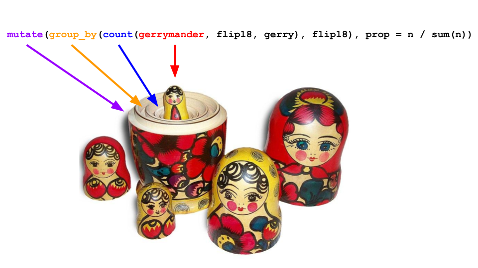
`mutate()`

Flip the question

Note

Is a Congressional District more likely to have high prevalence of gerrymandering if a Democrat was able to flip the seat in the 2018 election?

vs.

Note

Is a Congressional District more likely to be flipped to a Democratic seat if it has high prevalence of gerrymandering or low prevalence of gerrymandering?

Flipping vs. gerrymandering prevalence

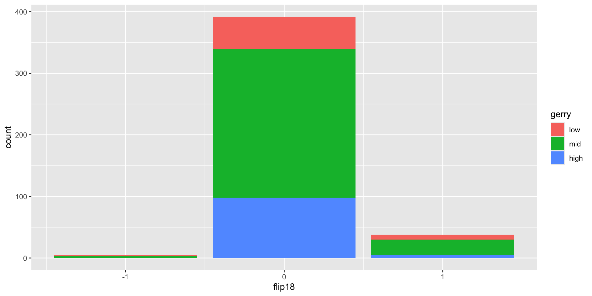
The following code should produce a visualization that answers the question “Is a Congressional District more likely to be flipped to a Democratic seat if it has high prevalence of gerrymandering or low prevalence of gerrymandering?” However, it produces a warning and an unexpected plot. What’s going on?

ggplot(
  gerrymander, 
  aes(x = gerry, fill = flip18)
  ) +
  geom_bar(position = "fill")

Warning: The following aesthetics were dropped during statistical transformation: fill.
ℹ This can happen when ggplot fails to infer the correct grouping structure in
  the data.
ℹ Did you forget to specify a `group` aesthetic or to convert a numerical
  variable into a factor?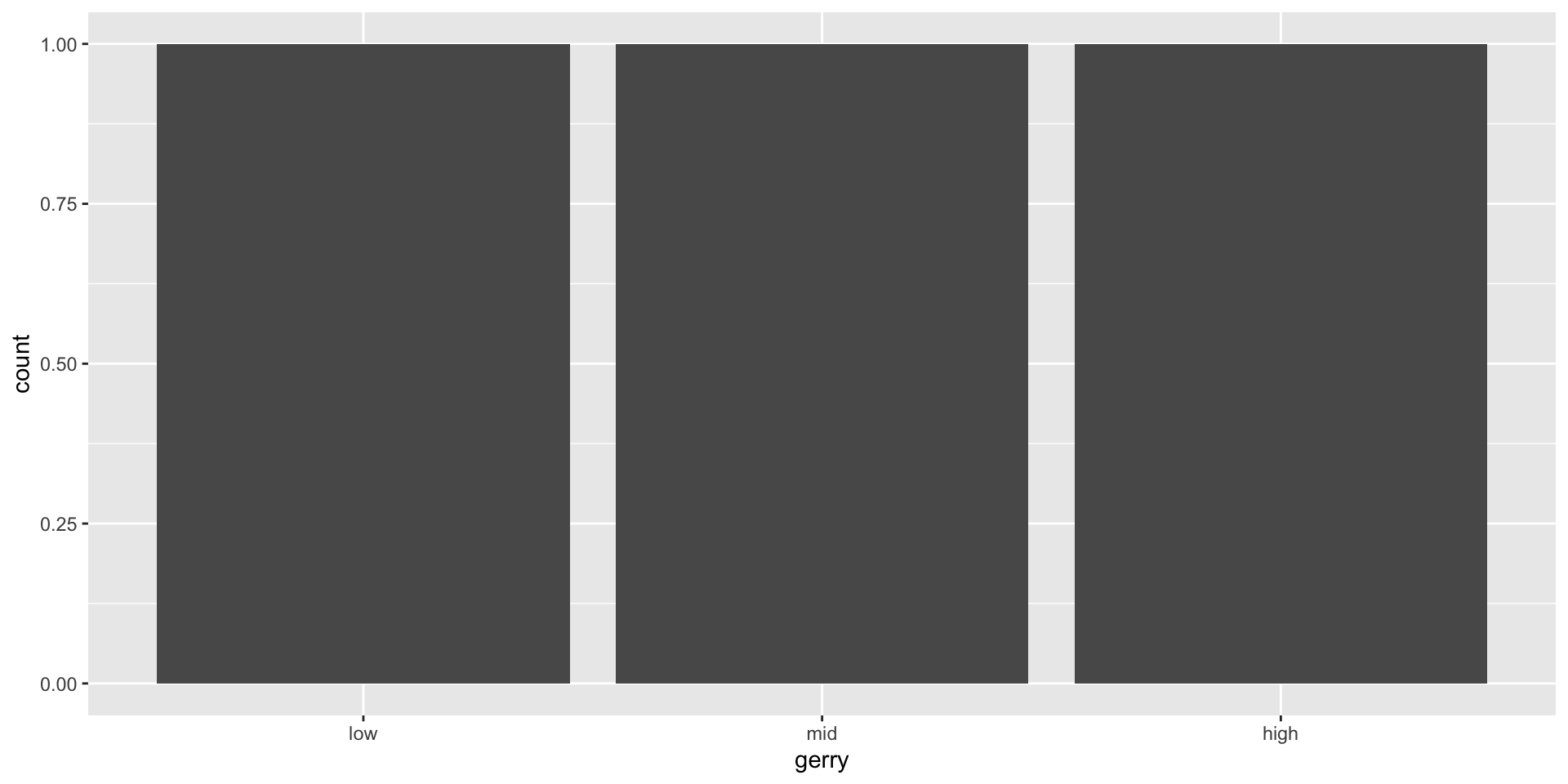

Another glimpse at `gerrymander`

glimpse(gerrymander)

Rows: 435
Columns: 12
$ district   <chr> "AK-AL", "AL-01", "AL-02", "AL-03", "AL-04", "AL-05", "AL-0…
$ last_name  <chr> "Young", "Byrne", "Roby", "Rogers", "Aderholt", "Brooks", "…
$ first_name <chr> "Don", "Bradley", "Martha", "Mike D.", "Rob", "Mo", "Gary",…
$ party16    <chr> "R", "R", "R", "R", "R", "R", "R", "D", "R", "R", "R", "R",…
$ clinton16  <dbl> 37.6, 34.1, 33.0, 32.3, 17.4, 31.3, 26.1, 69.8, 30.2, 41.7,…
$ trump16    <dbl> 52.8, 63.5, 64.9, 65.3, 80.4, 64.7, 70.8, 28.6, 65.0, 52.4,…
$ dem16      <dbl> 0, 0, 0, 0, 0, 0, 0, 1, 0, 0, 0, 0, 1, 0, 1, 0, 0, 0, 1, 0,…
$ state      <chr> "AK", "AL", "AL", "AL", "AL", "AL", "AL", "AL", "AR", "AR",…
$ party18    <chr> "R", "R", "R", "R", "R", "R", "R", "D", "R", "R", "R", "R",…
$ dem18      <dbl> 0, 0, 0, 0, 0, 0, 0, 1, 0, 0, 0, 0, 1, 1, 1, 0, 0, 0, 1, 0,…
$ flip18     <dbl> 0, 0, 0, 0, 0, 0, 0, 0, 0, 0, 0, 0, 0, 1, 0, 0, 0, 0, 0, 0,…
$ gerry      <fct> mid, high, high, high, high, high, high, high, mid, mid, mi…

`mutate()`

We want to use flip18 as a categorical variable
But it’s stored as a numeric
So we need to change its type first, before we can use it as a categorical variable
The mutate() function transforms (mutates) a data frame by creating a new column or updating an existing one

`mutate()` in action

gerrymander |>
  mutate(flip18 = as.factor(flip18))

# A tibble: 435 × 12
   district last_name first_name party16 clinton16 trump16 dem16 state party18
   <chr>    <chr>     <chr>      <chr>       <dbl>   <dbl> <dbl> <chr> <chr>  
 1 AK-AL    Young     Don        R            37.6    52.8     0 AK    R      
 2 AL-01    Byrne     Bradley    R            34.1    63.5     0 AL    R      
 3 AL-02    Roby      Martha     R            33      64.9     0 AL    R      
 4 AL-03    Rogers    Mike D.    R            32.3    65.3     0 AL    R      
 5 AL-04    Aderholt  Rob        R            17.4    80.4     0 AL    R      
 6 AL-05    Brooks    Mo         R            31.3    64.7     0 AL    R      
 7 AL-06    Palmer    Gary       R            26.1    70.8     0 AL    R      
 8 AL-07    Sewell    Terri      D            69.8    28.6     1 AL    D      
 9 AR-01    Crawford  Rick       R            30.2    65       0 AR    R      
10 AR-02    Hill      French     R            41.7    52.4     0 AR    R      
# ℹ 425 more rows
# ℹ 3 more variables: dem18 <dbl>, flip18 <fct>, gerry <fct>

`mutate()` in action

gerrymander |>
  mutate(flip18 = as.factor(flip18)) |>
  relocate(flip18)

# A tibble: 435 × 12
   flip18 district last_name first_name party16 clinton16 trump16 dem16 state
   <fct>  <chr>    <chr>     <chr>      <chr>       <dbl>   <dbl> <dbl> <chr>
 1 0      AK-AL    Young     Don        R            37.6    52.8     0 AK   
 2 0      AL-01    Byrne     Bradley    R            34.1    63.5     0 AL   
 3 0      AL-02    Roby      Martha     R            33      64.9     0 AL   
 4 0      AL-03    Rogers    Mike D.    R            32.3    65.3     0 AL   
 5 0      AL-04    Aderholt  Rob        R            17.4    80.4     0 AL   
 6 0      AL-05    Brooks    Mo         R            31.3    64.7     0 AL   
 7 0      AL-06    Palmer    Gary       R            26.1    70.8     0 AL   
 8 0      AL-07    Sewell    Terri      D            69.8    28.6     1 AL   
 9 0      AR-01    Crawford  Rick       R            30.2    65       0 AR   
10 0      AR-02    Hill      French     R            41.7    52.4     0 AR   
# ℹ 425 more rows
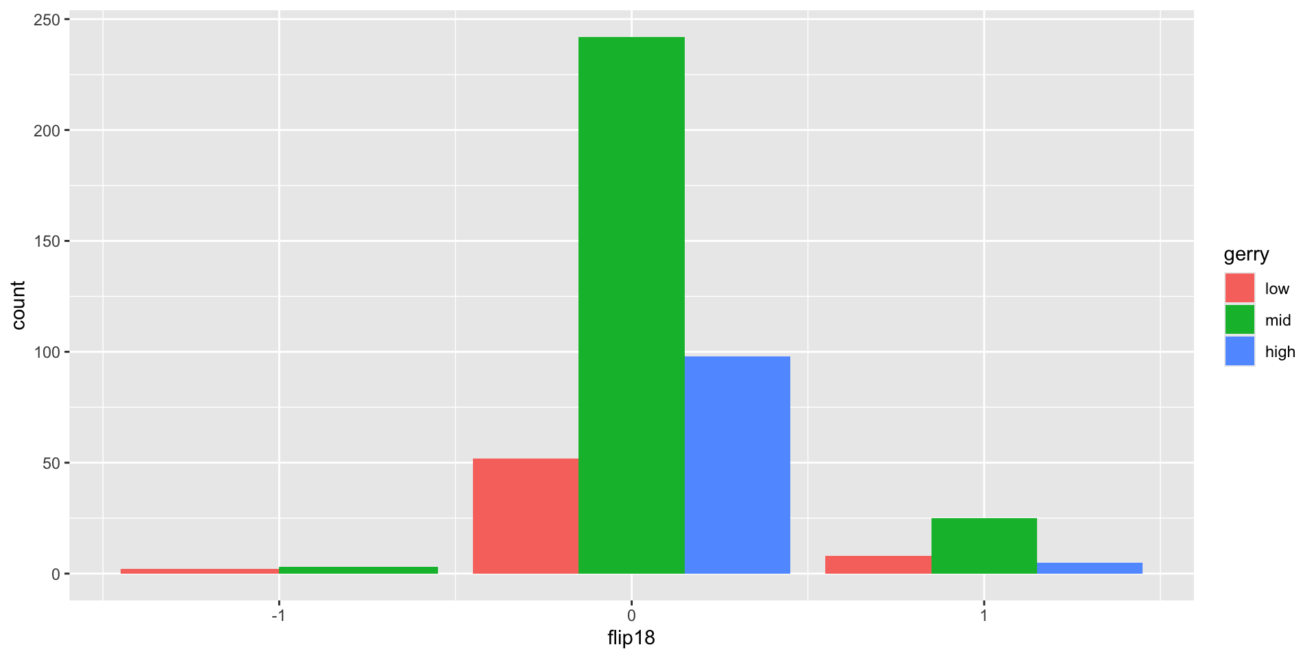
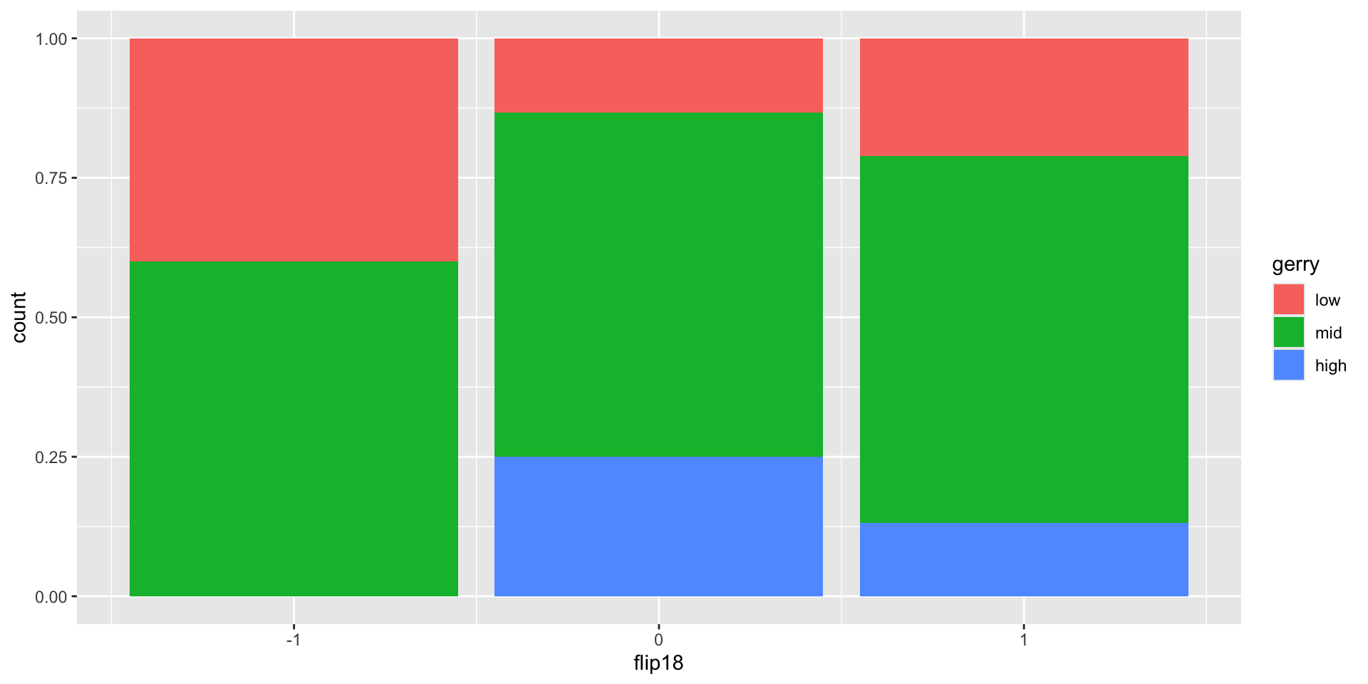
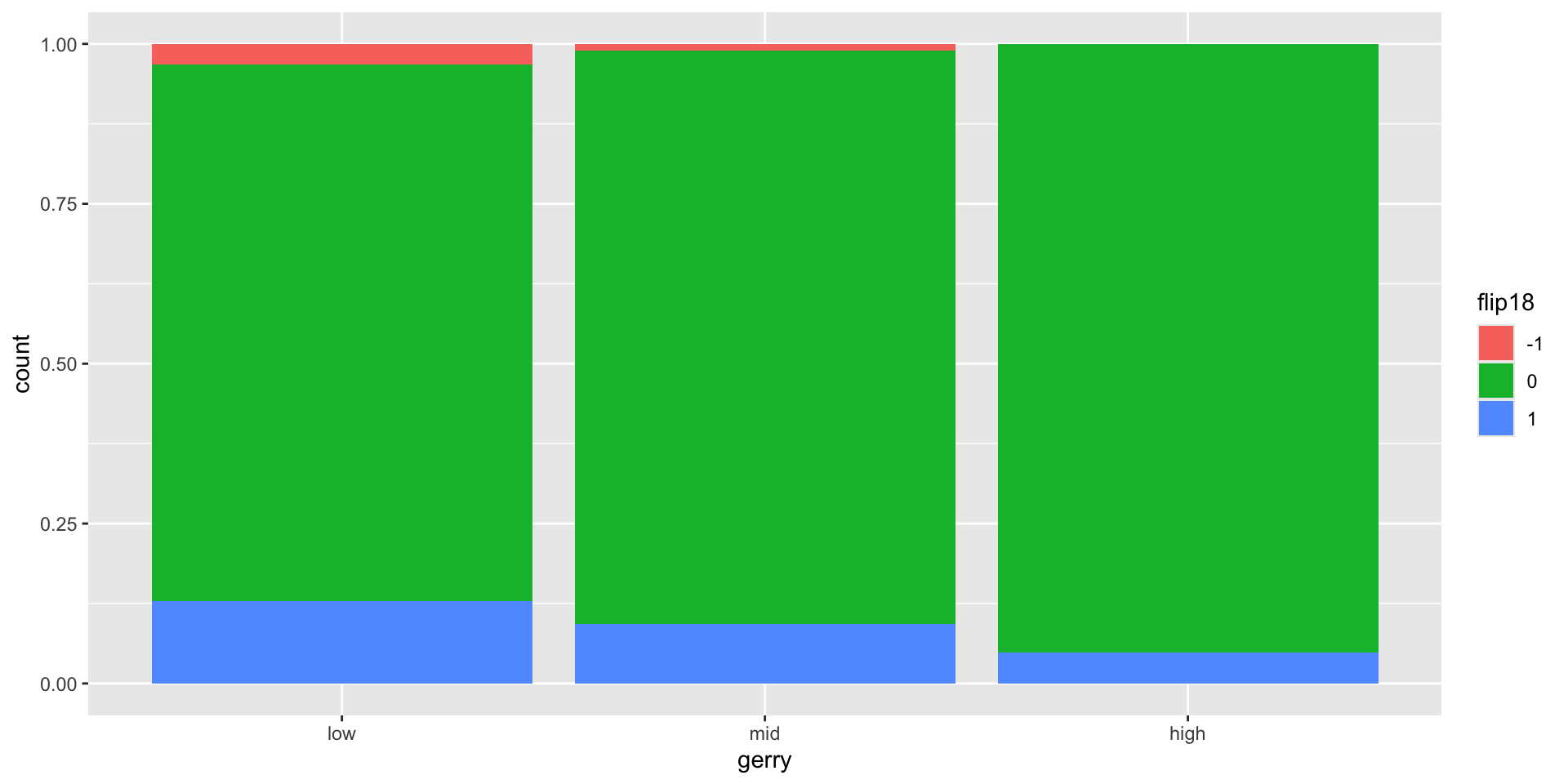
# ℹ 3 more variables: party18 <chr>, dem18 <dbl>, gerry <fct>

Revisit the plot

“Is a Congressional District more likely to be flipped to a Democratic seat if it has high prevalence of gerrymandering or low prevalence of gerrymandering?”

gerrymander |>
  mutate(flip18 = as.factor(flip18)) |>
  ggplot(aes(x = gerry, fill = flip18)) +
  geom_bar(position = "fill")

Application exercise

ae-04-gerrymander-explore-II

Go to your ae project in RStudio.
If you haven’t yet done so, make sure all of your changes up to this point are committed and pushed, i.e., there’s nothing left in your Git pane.
If you haven’t yet done so, click Pull to get today’s application exercise file: ae-04-gerrymander-explore-II.qmd.
Work through the application exercise in class, and render, commit, and push your edits by the end of class.

Recap: aesthetic mappings

Local aesthetic mappings for a given geom
Global aesthetic mappings for all geoms

Exploring data II

Warm-up

While you wait…

Intro to Coding Principles with Dav King

Reminder: Lab guidelines

Code style and readability

gerrymander

Packages

From last time

From last time

From last time

From last time

Step 1

Step 2

Step 3

Step 4

Same thing, without the pipe

With the pipe

Without the pipe

group_by(), summarize(), count()

What does group_by() do?

What does group_by() do?

Let’s simplify!

Let’s simplify!

group_by()

group_by()

group_by() |> summarize()

group_by() |> summarize()

summarize()

Spot the difference

count()

count() and sort

count() and sort

count() and sort

mutate()

Flip the question

Flipping vs. gerrymandering prevalence

Another glimpse at gerrymander

mutate()

mutate() in action

mutate() in action

Revisit the plot

Application exercise

ae-04-gerrymander-explore-II

Recap: aesthetic mappings

`gerrymander`

`group_by()`, `summarize()`, `count()`

What does `group_by()` do?

What does `group_by()` do?

`group_by()`

`group_by()`

`group_by() |> summarize()`

`group_by() |> summarize()`

`summarize()`

`count()`

`count()` and `sort`

`count()` and `sort`

`count()` and `sort`

`mutate()`

Another glimpse at `gerrymander`

`mutate()`

`mutate()` in action

`mutate()` in action