Tidying data

Lecture 6

John Zito

Duke University
STA 199 Spring 2025

2025-01-30

Warm-up

While you wait…

Prepare for today’s application exercise: ae-05-majors-tidy

Go to your ae project in RStudio.
Make sure all of your changes up to this point are committed and pushed, i.e., there’s nothing left in your Git pane.
Click Pull to get today’s application exercise file: ae-05-majors-tidy.qmd.
Wait till the you’re prompted to work on the application exercise during class before editing the file.

AEs are due by the end of class

Successful completion means at least one commit + push by 2PM today

Intro to Coding Principles with Dav King

8:30 PM Tonight!;
Social Sciences 139;
Space is limited, so please sign up;
Materials will be posted afterward;
We might do more if there is interest and Dav is available.

:::

Syllabus clarifications

You can miss 30% of AEs before it starts affecting your final grade. This policy is meant to smooth over technical mishaps, absences due to illness, athletics, etc. So we’re generally not granting extensions or exemptions. Just let the 30% policy do its thing;
ChatGPT: Thank (most of) you for citing! But please do not just dump the question verbatim into the chat. It irritates my valve;
Lab grade includes workflow points:
- Git was configured successfully such that a GitHub name is associated with the commit on GitHub (i.e., did Lab 0 successfully).
- PDF exists in GitHub repo for lab.
- At least 3 commits were made and pushed to the GitHub repo for lab.

Miscellany: logical operators

Generally useful in a filter() but will come up in various other places as well…

operator	definition
`<`	is less than?
`<=`	is less than or equal to?
`>`	is greater than?
`>=`	is greater than or equal to?
`==`	is exactly equal to?
`!=`	is not equal to?

Miscellany: logical operators (cont.)

Generally useful in a filter() but will come up in various other places as well…

operator	definition
`x & y`	is x AND y?
`x \| y`	is x OR y?
`is.na(x)`	is x NA?
`!is.na(x)`	is x not NA?
`x %in% y`	is x in y?
`!(x %in% y)`	is x not in y?
`!x`	is not x? (only makes sense if `x` is `TRUE` or `FALSE`)

Miscellany: assignment

Let’s make a tiny data frame to use as an example:

df <- tibble(x = c(1, 2, 3, 4, 5), y = c("a", "a", "b", "c", "c"))
df

# A tibble: 5 × 2
      x y    
  <dbl> <chr>
1     1 a    
2     2 a    
3     3 b    
4     4 c    
5     5 c

Miscellany: assignment

Suppose you run the following and then you inspect df, will the x variable have values 1, 2, 3, 4, 5 or 2, 4, 6, 8, 10?

df |>
  mutate(x = x * 2)

# A tibble: 5 × 2
      x y    
  <dbl> <chr>
1     2 a    
2     4 a    
3     6 b    
4     8 c    
5    10 c

df

Miscellany: assignment

Suppose you run the following and then you inspect df, will the x variable have values 1, 2, 3, 4, 5 or 2, 4, 6, 8, 10?

df |>
  mutate(x = x * 2)

# A tibble: 5 × 2
      x y    
  <dbl> <chr>
1     2 a    
2     4 a    
3     6 b    
4     8 c    
5    10 c

df

# A tibble: 5 × 2
      x y    
  <dbl> <chr>
1     1 a    
2     2 a    
3     3 b    
4     4 c    
5     5 c

Do something and show me

Miscellany: assignment

Suppose you run the following and then you inspect df, will the x variable has values 1, 2, 3, 4, 5 or 2, 4, 6, 8, 10?

df <- df |>
  mutate(x = x * 2)

df

Miscellany: assignment

Suppose you run the following and then you inspect df, will the x variable has values 1, 2, 3, 4, 5 or 2, 4, 6, 8, 10?

df <- df |>
  mutate(x = x * 2)

df

# A tibble: 5 × 2
      x y    
  <dbl> <chr>
1     2 a    
2     4 a    
3     6 b    
4     8 c    
5    10 c

Do something and save result

Miscellany: assignment

Do something, save result, overwriting original

df <- tibble(
  x = c(1, 2, 3, 4, 5), 
  y = c("a", "a", "b", "c", "c")
)
df <- df |>
  mutate(x = x * 2)
df

# A tibble: 5 × 2
      x y    
  <dbl> <chr>
1     2 a    
2     4 a    
3     6 b    
4     8 c    
5    10 c

Do something, save result, not overwriting original

df <- tibble(
  x = c(1, 2, 3, 4, 5), 
  y = c("a", "a", "b", "c", "c")
)
df_new <- df |>
  mutate(x = x * 2)
df_new

# A tibble: 5 × 2
      x y    
  <dbl> <chr>
1     2 a    
2     4 a    
3     6 b    
4     8 c    
5    10 c

Miscellany: assignment

Do something, save result, overwriting original when you shouldn’t

df <- tibble(
  x = c(1, 2, 3, 4, 5), 
  y = c("a", "a", "b", "c", "c")
)
df <- df |>
  group_by(y) |>
  summarize(mean_x = mean(x))
df

# A tibble: 3 × 2
  y     mean_x
  <chr>  <dbl>
1 a        1.5
2 b        3  
3 c        4.5

Do something, save result, not overwriting original when you shouldn’t

df <- tibble(
  x = c(1, 2, 3, 4, 5), 
  y = c("a", "a", "b", "c", "c")
)
df_summary <- df |>
  group_by(y) |>
  summarize(mean_x = mean(x))
df_summary

# A tibble: 3 × 2
  y     mean_x
  <chr>  <dbl>
1 a        1.5
2 b        3  
3 c        4.5

Miscellany: assignment

Do something, save result, overwriting original
data frame

df <- tibble(
  x = c(1, 2, 3, 4, 5), 
  y = c("a", "a", "b", "c", "c")
)
df <- df |>
  mutate(z = x + 2)
df

# A tibble: 5 × 3
      x y         z
  <dbl> <chr> <dbl>
1     1 a         3
2     2 a         4
3     3 b         5
4     4 c         6
5     5 c         7

Do something, save result, overwriting original
column

df <- tibble(
  x = c(1, 2, 3, 4, 5), 
  y = c("a", "a", "b", "c", "c")
)
df <- df |>
  mutate(x = x + 2)
df

# A tibble: 5 × 2
      x y    
  <dbl> <chr>
1     3 a    
2     4 a    
3     5 b    
4     6 c    
5     7 c

Data tidying

Tidy data

“Tidy datasets are easy to manipulate, model and visualise, and have a specific structure: each variable is a column, each observation is a row, and each type of observational unit is a table.”

Tidy Data, https://vita.had.co.nz/papers/tidy-data.pdf

Note: “easy to manipulate” = “straightforward to manipulate”

Goal

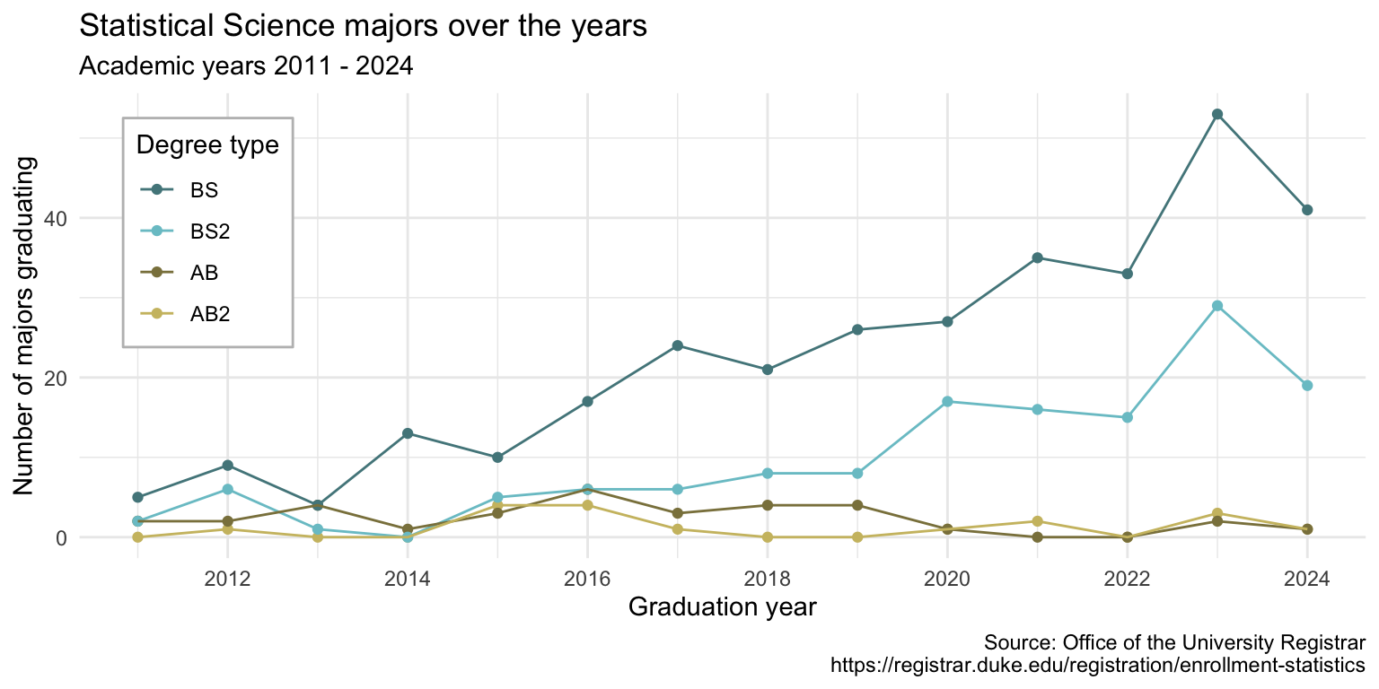
Visualize StatSci majors over the years!

Data

statsci <- read_csv("data/statsci.csv")
statsci

# A tibble: 4 × 15
  degree   `2011` `2012` `2013` `2014` `2015` `2016` `2017` `2018` `2019` `2020`
  <chr>     <dbl>  <dbl>  <dbl>  <dbl>  <dbl>  <dbl>  <dbl>  <dbl>  <dbl>  <dbl>
1 Statist…     NA      1     NA     NA      4      4      1     NA     NA      1
2 Statist…      2      2      4      1      3      6      3      4      4      1
3 Statist…      2      6      1     NA      5      6      6      8      8     17
4 Statist…      5      9      4     13     10     17     24     21     26     27
# ℹ 4 more variables: `2021` <dbl>, `2022` <dbl>, `2023` <dbl>, `2024` <dbl>

The first column (variable) is the degree, and there are 4 possible degrees: BS (Bachelor of Science), BS2 (Bachelor of Science, 2nd major), AB (Bachelor of Arts), AB2 (Bachelor of Arts, 2nd major).
The remaining columns show the number of students graduating with that major in a given academic year from 2011 to 2024.

Let’s plan!

In a perfect world, how would our data be formatted to create this plot? What do the columns need to be? What would go inside aes when we call ggplot?

The goal

We want to be able to write code that starts something like this:

ggplot(statsci, aes(x = year, y = n, color = degree_type)) + 
  ...

But the data are not in a format that will allow us to do that.

The challenge

How do we go from this…

# A tibble: 4 × 8
  degree `2011` `2012` `2013` `2014` `2015` `2016` `2017`
  <fct>   <dbl>  <dbl>  <dbl>  <dbl>  <dbl>  <dbl>  <dbl>
1 AB2        NA      1     NA     NA      4      4      1
2 AB          2      2      4      1      3      6      3
3 BS2         2      6      1     NA      5      6      6
4 BS          5      9      4     13     10     17     24

…to this?

# A tibble: 56 × 3
   degree_type  year     n
   <fct>       <dbl> <dbl>
 1 AB2          2011     0
 2 AB2          2012     1
 3 AB2          2013     0
 4 AB2          2014     0
 5 AB2          2015     4
 6 AB2          2016     4
 7 AB2          2017     1
 8 AB2          2018     0
 9 AB2          2019     0
10 AB2          2020     1
11 AB2          2021     2
12 AB2          2022     0
13 AB2          2023     3
14 AB2          2024     1
15 AB           2011     2
16 AB           2012     2
# ℹ 40 more rows

With the command pivot_longer()!

`pivot_longer()`

Pivot the statsci data frame longer such that each row represents a degree type / year combination and year and number of graduates for that year are columns in the data frame.

statsci |>
  pivot_longer(
    cols = -degree,
    names_to = "year",
    values_to = "n"
  )

# A tibble: 56 × 3
   degree                    year      n
   <chr>                     <chr> <dbl>
 1 Statistical Science (AB2) 2011     NA
 2 Statistical Science (AB2) 2012      1
 3 Statistical Science (AB2) 2013     NA
 4 Statistical Science (AB2) 2014     NA
 5 Statistical Science (AB2) 2015      4
 6 Statistical Science (AB2) 2016      4
 7 Statistical Science (AB2) 2017      1
 8 Statistical Science (AB2) 2018     NA
 9 Statistical Science (AB2) 2019     NA
10 Statistical Science (AB2) 2020      1
# ℹ 46 more rows

`year`

What is the type of the year variable? Why? What should it be?

It’s a character (chr) variable since the information came from the columns of the original data frame and R cannot know that these character strings represent years. The variable type should be numeric.

`pivot_longer()` again

Start over with pivoting, and this time also make sure year is a numerical variable in the resulting data frame.

statsci |>
  pivot_longer(
    cols = -degree,
    names_to = "year",
    values_to = "n",
    names_transform = as.numeric,
  )

# A tibble: 56 × 3
   degree                     year     n
   <chr>                     <dbl> <dbl>
 1 Statistical Science (AB2)  2011    NA
 2 Statistical Science (AB2)  2012     1
 3 Statistical Science (AB2)  2013    NA
 4 Statistical Science (AB2)  2014    NA
 5 Statistical Science (AB2)  2015     4
 6 Statistical Science (AB2)  2016     4
 7 Statistical Science (AB2)  2017     1
 8 Statistical Science (AB2)  2018    NA
 9 Statistical Science (AB2)  2019    NA
10 Statistical Science (AB2)  2020     1
# ℹ 46 more rows

`NA` counts

What does an NA mean in this context? Hint: The data come from the university registrar, and they have records on every single graduates, there shouldn’t be anything “unknown” to them about who graduated when.

NAs should actually be 0s.

Clean-up

Add on to your pipeline that you started with pivoting and convert NAs in n to 0s.

statsci |>
  pivot_longer(
    cols = -degree,
    names_to = "year",
    names_transform = as.numeric,
    values_to = "n"
  ) |>
  mutate(n = if_else(is.na(n), 0, n))

# A tibble: 56 × 3
   degree                     year     n
   <chr>                     <dbl> <dbl>
 1 Statistical Science (AB2)  2011     0
 2 Statistical Science (AB2)  2012     1
 3 Statistical Science (AB2)  2013     0
 4 Statistical Science (AB2)  2014     0
 5 Statistical Science (AB2)  2015     4
 6 Statistical Science (AB2)  2016     4
 7 Statistical Science (AB2)  2017     1
 8 Statistical Science (AB2)  2018     0
 9 Statistical Science (AB2)  2019     0
10 Statistical Science (AB2)  2020     1
# ℹ 46 more rows

More clean-up

In our plot the degree types are BS, BS2, AB, and AB2. This information is in our dataset, in the degree column, but this column also has additional characters we don’t need. Create a new column called degree_type with levels BS, BS2, AB, and AB2 (in this order) based on degree. Do this by adding on to your pipeline from earlier.

statsci |>
  pivot_longer(
    cols = -degree,
    names_to = "year",
    names_transform = as.numeric,
    values_to = "n"
  ) |>
  mutate(n = if_else(is.na(n), 0, n)) |>
  separate(degree, sep = " \\(", into = c("major", "degree_type")) |>
  mutate(
    degree_type = str_remove(degree_type, "\\)"),
    degree_type = fct_relevel(degree_type, "BS", "BS2", "AB", "AB2")
  )

# A tibble: 56 × 4
   major               degree_type  year     n
   <chr>               <fct>       <dbl> <dbl>
 1 Statistical Science AB2          2011     0
 2 Statistical Science AB2          2012     1
 3 Statistical Science AB2          2013     0
 4 Statistical Science AB2          2014     0
 5 Statistical Science AB2          2015     4
 6 Statistical Science AB2          2016     4
 7 Statistical Science AB2          2017     1
 8 Statistical Science AB2          2018     0
 9 Statistical Science AB2          2019     0
10 Statistical Science AB2          2020     1
# ℹ 46 more rows

Finish

Now that you have your data pivoting and cleaning pipeline figured out, save the resulting data frame as statsci_longer.

statsci_longer <- statsci |>
  pivot_longer(
    cols = -degree,
    names_to = "year",
    names_transform = as.numeric,
    values_to = "n"
  ) |>
  mutate(n = if_else(is.na(n), 0, n)) |>
  separate(degree, sep = " \\(", into = c("major", "degree_type")) |>
  mutate(
    degree_type = str_remove(degree_type, "\\)"),
    degree_type = fct_relevel(degree_type, "BS", "BS2", "AB", "AB2")
  )

ae-05-majors-tidy

Go to your ae project in RStudio.
If you haven’t yet done so, make sure all of your changes up to this point are committed and pushed, i.e., there’s nothing left in your Git pane.
If you haven’t yet done so, click Pull to get today’s application exercise file: ae-05-majors-tidy.qmd.
Work through the application exercise in class, and render, commit, and push your edits by the end of class.

Recap: pivoting

Data sets can’t be labeled as wide or long but they can be made wider or longer for a certain analysis that requires a certain format
When pivoting longer, variable names that turn into values are characters by default. If you need them to be in another format, you need to explicitly make that transformation, which you can do so within the pivot_longer() function.
You can tweak a plot forever, but at some point the tweaks are likely not very productive. However, you should always be critical of defaults (however pretty they might be) and see if you can improve the plot to better portray your data / results / what you want to communicate.

Tidying data

Warm-up

While you wait…

Intro to Coding Principles with Dav King

Syllabus clarifications

Miscellany: logical operators

Miscellany: logical operators (cont.)

Miscellany: assignment

Miscellany: assignment

Miscellany: assignment

Miscellany: assignment

Miscellany: assignment

Miscellany: assignment

Miscellany: assignment

Miscellany: assignment

Data tidying

Tidy data

Goal

Data

Let’s plan!

The goal

The challenge

pivot_longer()

year

pivot_longer() again

NA counts

Clean-up

More clean-up

Finish

ae-05-majors-tidy

Recap: pivoting

`pivot_longer()`

`year`

`pivot_longer()` again

`NA` counts