Importing and recoding data

Lecture 9

John Zito

Duke University
STA 199 Spring 2025

2025-02-11

While you wait…

Go to your ae project in RStudio.
Make sure all of your changes up to this point are committed and pushed, i.e., there’s nothing left in your Git pane.
Click Pull to get today’s application exercise file: ae-08-age-gaps-sales-import.qmd.
Wait till the you’re prompted to work on the application exercise during class before editing the file.

AEs are due by the end of class

Successful completion means at least one commit + push by 2PM today.

That pesky midterm…

Midterm Exam 1

Worth 20% of your final grade; consists of two parts:

In-class: worth 70% of the Midterm 1 grade;
- Thursday February 20 11:45 AM - 1:00 PM
Take-home: worth 30% of the Midterm 1 grade.
- Released Thursday February 20 at 1:00 PM;
- Due Monday February 24 at 8:30 AM.

In-class

All multiple choice;
You will take it in Bio Sciences 111 (this room) or Physics 128;
You get both sides of one 8.5” x 11” note sheet that you and only you created (written, typed, iPad, etc);
If you do better on the final than you do on this, the final exam score will replace this.

Important

If you have testing accommodations, make sure I get proper documentation from SDAO and make appointments in the Testing Center by Friday. The appointment should overlap substantially with our class time if possible.

Example in-class question

Which command will replace a pre-existing column in a data frame with a new and improved version of itself?

group_by
summarize
pivot_wider
geom_replace
mutate

Example in-class question

df

# A tibble: 6 × 2
      x y      
  <dbl> <chr>  
1     1 John   
2     2 John   
3     3 Cameron
4     4 Zito   
5     5 Zito   
6     6 Zito

df |>
  group_by(y) |>
  summarize(xbar = mean(x))

How many rows will this output have?

Example in-class question

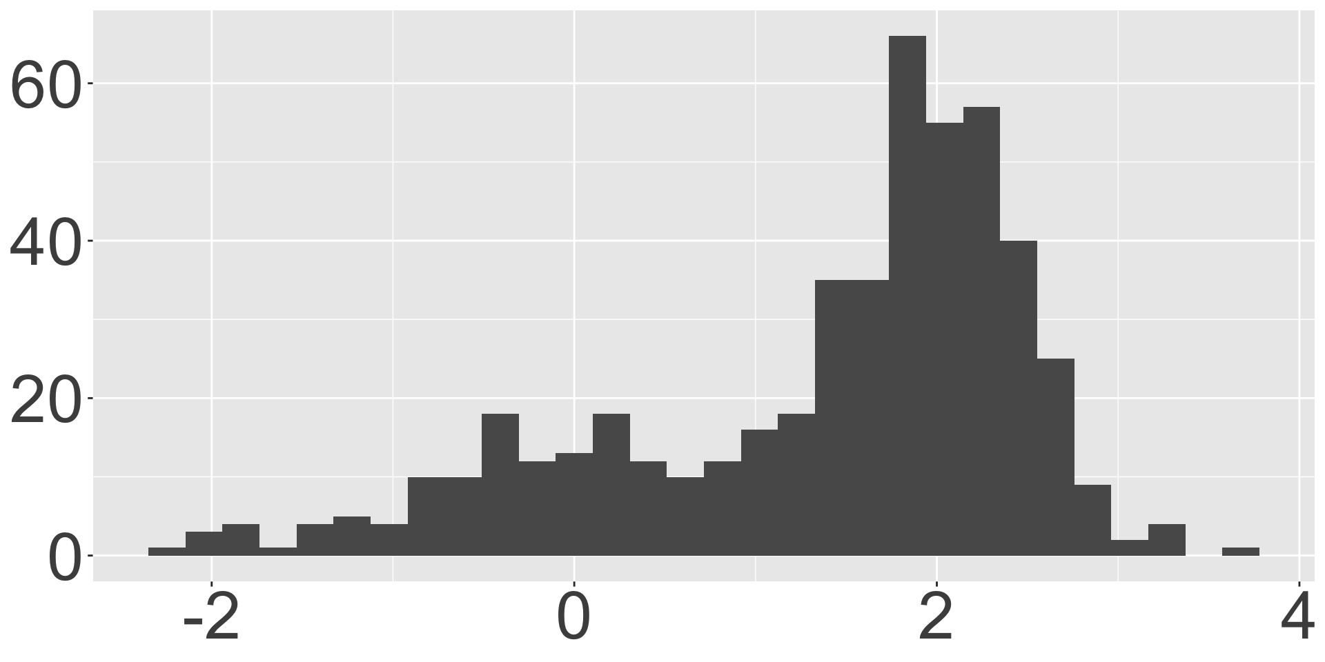
Which box plot is visualizing the same data as the histogram?

What should I put on my cheat sheet?

Ask one of our undergrad TAs! They took the class. I didn’t.

description of common functions;
description of different visualizations: how to interpret, and what to use when;
doodles;
cute words of affirmation.

Warning

Don’t waste space on the details of any specific applications or datasets we’ve seen (penguins, Bechdel, gerrymandering, midwest, etc). Anything we want you to know about a particular application will be introduced from scratch within the exam.

Take-home

It will be just like a lab, only shorter;
Completely open-resource, but citation policies apply;
Absolutely no collaboration of any kind;
Seek help by posting privately on Ed;
Submit your final PDF to Gradescope in the usual way.

Reminder: conduct policies

Uncited use of outside resources or inappropriate collaboration will result in a zero and be referred to the conduct office;
If a conduct violation of any kind is discovered, your final letter grade in the course will be permanently reduced (A- down to B+, B+ down to B, etc);
If folks share solutions, all students involved will be penalized equally, the sharer the same as the recipient.

It’s not personal.

These policies apply to everyone. I don’t care who your parents are, or what medical schools you are applying to in the fall. Grow up and act right.

Things you can do to study

Practice problems: released Thursday February 13;
Attend lab: review game on Monday February 17;
Old labs: correct parts where you lost points;
Old AEs: complete tasks we didn’t get to and compare with key;
Code along: watch these videos specifically;
Textbook: odd-numbered exercises in the back of Chs. 1, 4, 5, 6.

Let’s zoom out for a sec…

Data science and statistical thinking

Before Midterm 1…

Data science: the real-world art of transforming messy, imperfect, incomplete data into knowledge;

After Midterm 1…

Statistics: the mathematical discipline of quantifying our uncertainty about that knowledge.

Data science

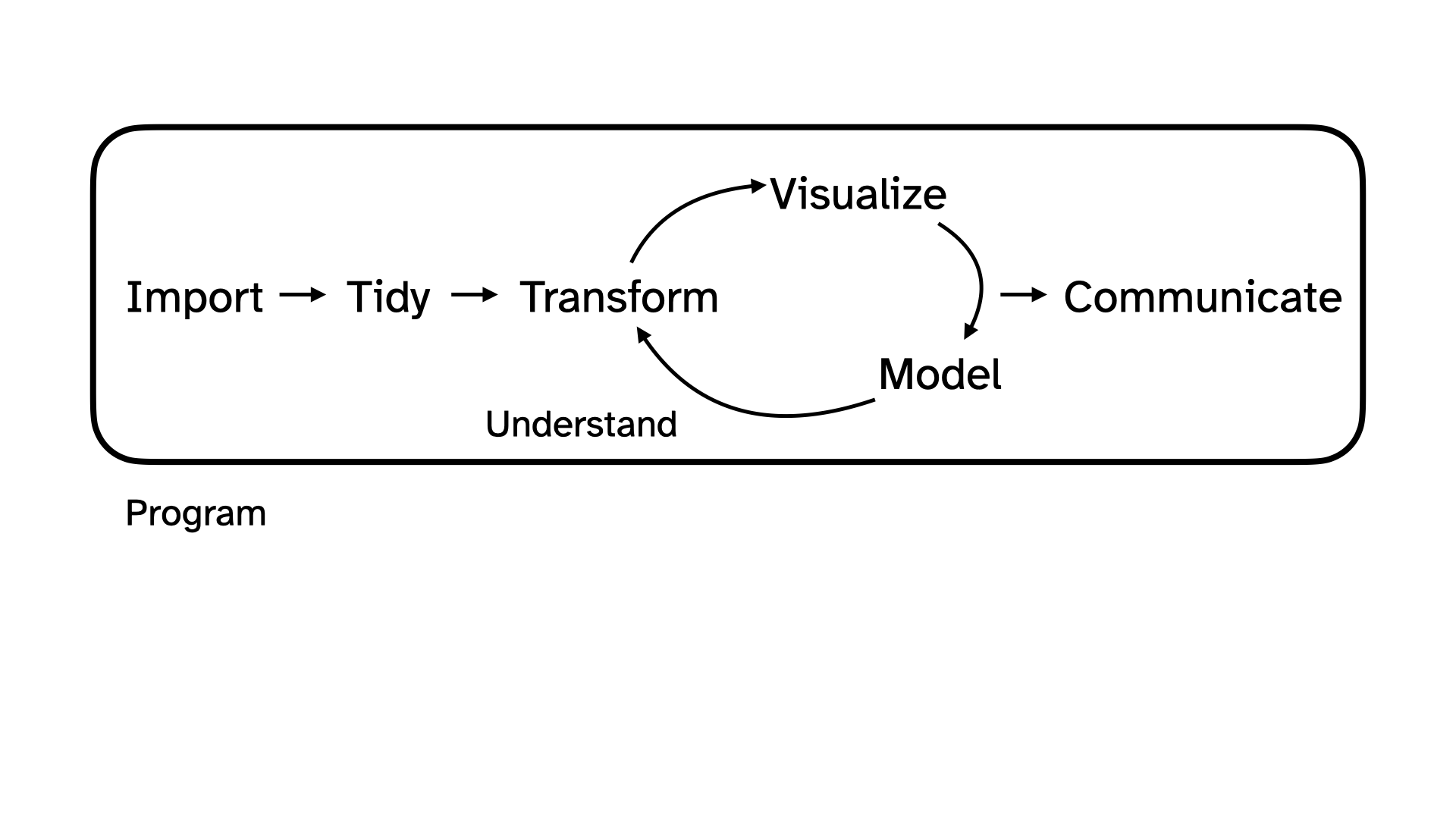
Data science

Collection: we won’t seriously study this!
- for us: data importing (read_csv), and webscraping (next time);
- but really: domain-specific issues of measurement, survey design, experimental design, etc;

From last time: data collection

I sent out my lil’ survey with Google Forms, downloaded the responses in a CSV, and read that sucker in:

survey <- read_csv("data/survey-2025-02-06.csv")
survey

# A tibble: 209 × 3
   Timestamp         How many classes do you have on Tues…¹ `What year are you?`
   <chr>             <chr>                                  <chr>               
 1 2/6/2025 11:33:57 3                                      Sophomore           
 2 2/6/2025 11:37:39 3                                      First-year          
 3 2/6/2025 11:40:55 2                                      Senior              
 4 2/6/2025 11:42:05 3                                      First-year          
 5 2/6/2025 11:42:46 3                                      Senior              
 6 2/6/2025 11:43:28 3                                      Senior              
 7 2/6/2025 11:44:41 3                                      First-year          
 8 2/6/2025 11:44:49 3                                      First-year          
 9 2/6/2025 11:44:51 2                                      Sophomore           
10 2/6/2025 11:44:51 3                                      Sophomore           
# ℹ 199 more rows
# ℹ abbreviated name: ¹`How many classes do you have on Tuesdays?`

Data science

Collection: we won’t seriously study this!
- for us: data importing (read_csv), and webscraping (next time);
- but really: domain-specific issues of measurement, survey design, experimental design, etc;

Preparation: cleaning, wrangling, and otherwise tidying the data so we can actually work with it.
- keywords: mutate, fct_relevel, pivot_*, *_join

From last time: data preparation

survey <- survey |>
  rename(
    tue_classes = `How many classes do you have on Tuesdays?`,
    year = `What year are you?`
  ) |>
  mutate(
    tue_classes = case_when(
      tue_classes == "2 -3" ~ "3",
      tue_classes == "3 classes" ~ "3",
      tue_classes == "Four" ~ "4",
      tue_classes == "TWO MANY" ~ "2",
      tue_classes == "Three" ~ "3",
      tue_classes == "Two" ~ "2",
      tue_classes == "Two plus a chemistry lab" ~ "3",
      tue_classes == "three" ~ "3",
      .default = tue_classes
    ),
    tue_classes = as.numeric(tue_classes),
    year = fct_relevel(year, "First-year", "Sophomore", "Junior", "Senior")
  ) |>
  select(tue_classes, year)
survey

# A tibble: 209 × 2
   tue_classes year      
         <dbl> <fct>     
 1           3 Sophomore 
 2           3 First-year
 3           2 Senior    
 4           3 First-year
 5           3 Senior    
 6           3 Senior    
 7           3 First-year
 8           3 First-year
 9           2 Sophomore 
10           3 Sophomore 
# ℹ 199 more rows

Data science

Collection: we won’t seriously study this!
- for us: data importing (read_csv), and webscraping (next time);
- but really: domain-specific issues of measurement, survey design, experimental design, etc;
Preparation: cleaning, wrangling, and otherwise tidying the data so we can actually work with it.
- keywords: mutate, fct_relevel, pivot_*, *_join

Analysis: finally transform the data into knowledge…
- pictures: ggplot, geom_*, etc
- numerical summaries: summarize, group_by, count, mean, median, sd, quantile, IQR, cor, etc

From last time: data analysis

A human being can learn nothing from staring at this box:

survey

# A tibble: 209 × 2
   tue_classes year      
         <dbl> <fct>     
 1           3 Sophomore 
 2           3 First-year
 3           2 Senior    
 4           3 First-year
 5           3 Senior    
 6           3 Senior    
 7           3 First-year
 8           3 First-year
 9           2 Sophomore 
10           3 Sophomore 
# ℹ 199 more rows

From last time: data analysis

Picture!

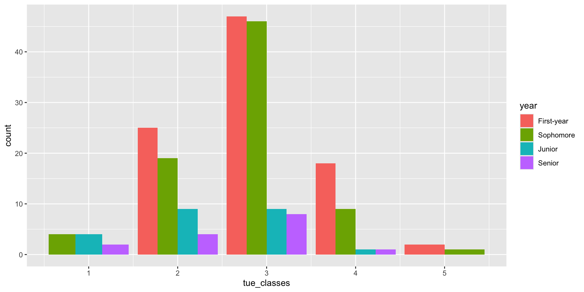
ggplot(survey, aes(x = tue_classes, fill = year)) + 
  geom_bar(position = "dodge")

From last time: data analysis

Better picture?

ggplot(survey, aes(x = tue_classes, fill = year)) + 
  geom_bar(position = "fill")

From last time: data analysis

Numbers!

survey |>
  count(tue_classes, year) |>
  group_by(tue_classes) |>
  mutate(prop = n / sum(n))

# A tibble: 17 × 4
# Groups:   tue_classes [5]
   tue_classes year           n   prop
         <dbl> <fct>      <int>  <dbl>
 1           1 Sophomore      4 0.4   
 2           1 Junior         4 0.4   
 3           1 Senior         2 0.2   
 4           2 First-year    25 0.439 
 5           2 Sophomore     19 0.333 
 6           2 Junior         9 0.158 
 7           2 Senior         4 0.0702
 8           3 First-year    47 0.427 
 9           3 Sophomore     46 0.418 
10           3 Junior         9 0.0818
11           3 Senior         8 0.0727
12           4 First-year    18 0.621 
13           4 Sophomore      9 0.310 
14           4 Junior         1 0.0345
15           4 Senior         1 0.0345
16           5 First-year     2 0.667 
17           5 Sophomore      1 0.333

Data science

Collection: we won’t seriously study this!
- for us: data importing (read_csv), and webscraping (next time);
- but really: domain-specific issues of measurement, survey design, experimental design, etc;
Preparation: cleaning, wrangling, and otherwise tidying the data so we can actually work with it.
- keywords: mutate, fct_relevel, pivot_*, *_join
Analysis: finally transform the data into knowledge…
- pictures: ggplot, geom_*, etc
- numerical summaries: summarize, group_by, count, mean, median, sd, quantile, iqr, cor, etc

The pictures and the summaries need to work together!

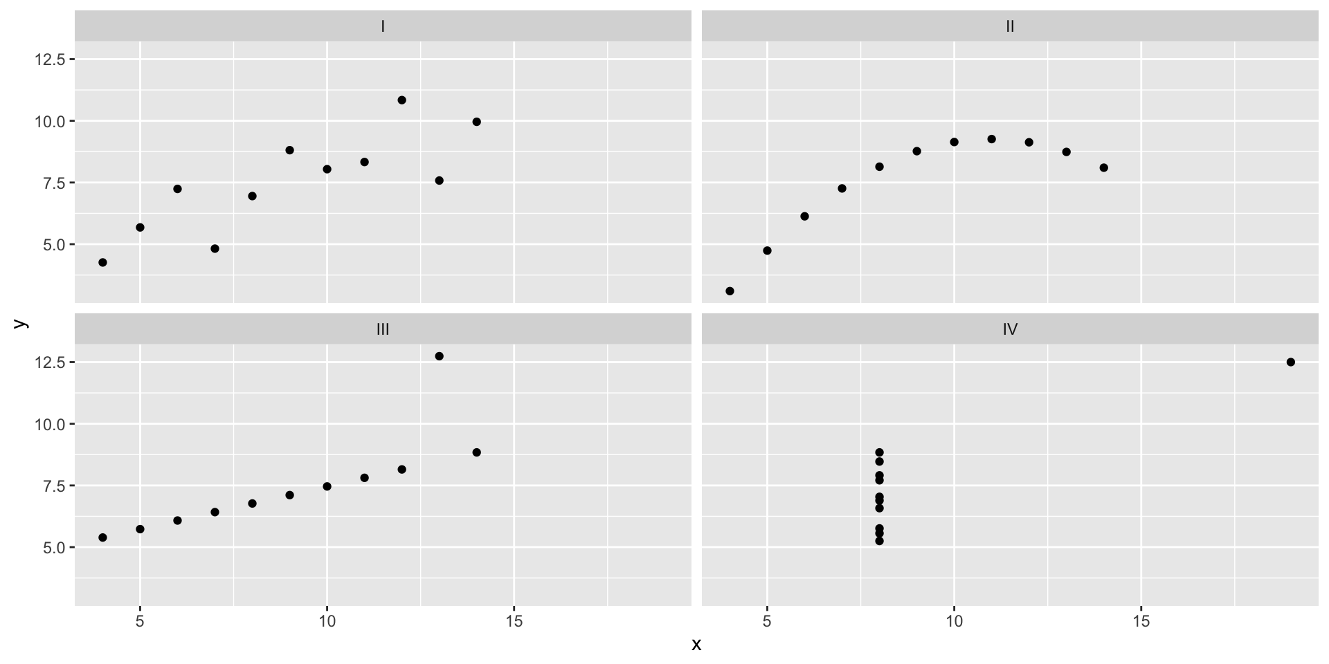
A cautionary tale: Anscombe’s quartet

Dataset I

    x     y
1  10  8.04
2   8  6.95
3  13  7.58
4   9  8.81
5  11  8.33
6  14  9.96
7   6  7.24
8   4  4.26
9  12 10.84
10  7  4.82
11  5  5.68

Dataset II

Dataset III

    x     y
1  10  7.46
2   8  6.77
3  13 12.74
4   9  7.11
5  11  7.81
6  14  8.84
7   6  6.08
8   4  5.39
9  12  8.15
10  7  6.42
11  5  5.73

Dataset IV

    x     y
1   8  6.58
2   8  5.76
3   8  7.71
4   8  8.84
5   8  8.47
6   8  7.04
7   8  5.25
8  19 12.50
9   8  5.56
10  8  7.91
11  8  6.89

A cautionary tale: Anscombe’s quartet

ggplot(anscombe_tidy, aes(x, y)) +
  geom_point() +
  facet_wrap(~ set)

A cautionary tale: Anscombe’s quartet

ggplot(anscombe_tidy, aes(x, y)) +
  geom_point() +
  facet_wrap(~ set) +
  geom_smooth(method = "lm", se = FALSE)

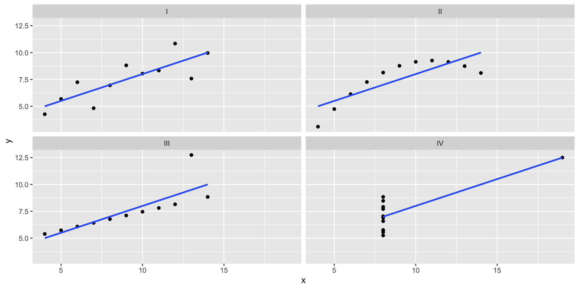
If you only looked at summary statistics…

anscombe_tidy |>
  group_by(set) |>
  summarize(
    xbar = mean(x),
    ybar = mean(y),
    sx = sd(x),
    sy = sd(y),
    r = cor(x, y)
  )

# A tibble: 4 × 6
  set    xbar  ybar    sx    sy     r
  <chr> <dbl> <dbl> <dbl> <dbl> <dbl>
1 I         9  7.50  3.32  2.03 0.816
2 II        9  7.50  3.32  2.03 0.816
3 III       9  7.5   3.32  2.03 0.816
4 IV        9  7.50  3.32  2.03 0.817

Our motto: ABV!

No, not alcohol by volume…

Always!
Be!
Visualizing!

From last time

Finish up: `ae-08-durham-climate-factors`

Go to your ae project in RStudio.
Open ae-08-durham-climate-factors.qmd and pick up at “Recode and reorder”.

Reading data into R

Reading rectangular data

Using readr:
- Most commonly: read_csv()
- Maybe also: read_tsv(), read_delim(), etc.

Using readxl: read_excel()

Using googlesheets4: read_sheet() – We haven’t covered this in the videos, but might be useful for your projects

Application exercise

Goal 1: Reading and writing CSV files

Read a CSV file
Split it into subsets based on features of the data
Write out subsets as CSV files

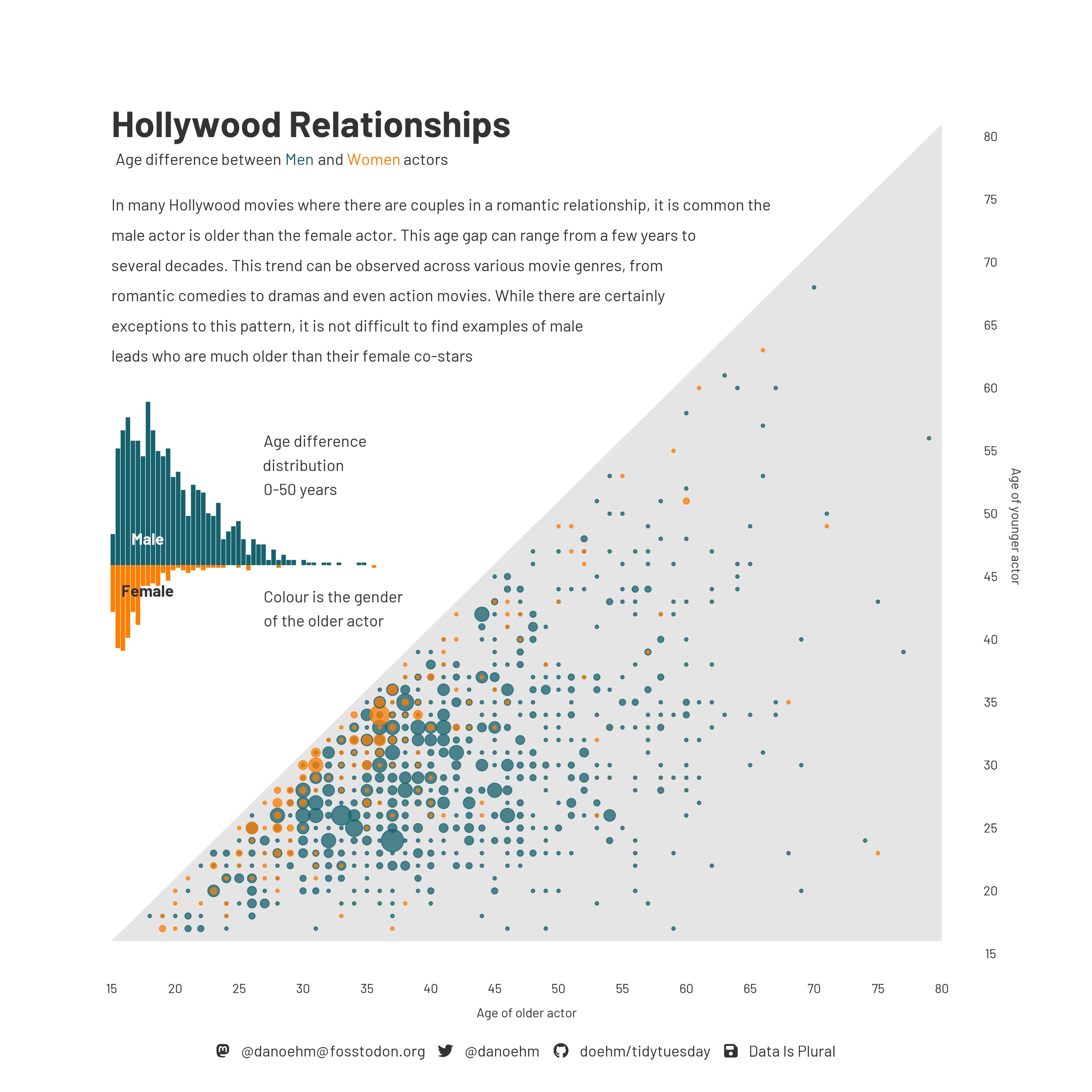
Age gap in Hollywood relationships

What is the story in this visualization?

ae-08-age-gaps-sales-import - Part 1

Go to your ae project in RStudio.
If you haven’t yet done so, make sure all of your changes up to this point are committed and pushed, i.e., there’s nothing left in your Git pane.
If you haven’t yet done so, click Pull to get today’s application exercise file: ae-08-age-gaps-sales-import.qmd.
Work through Part 1 of the application exercise in class, and render, commit, and push your edits.

Goal 2: Reading Excel files

Read an Excel file with non-tidy data
Tidy it up!

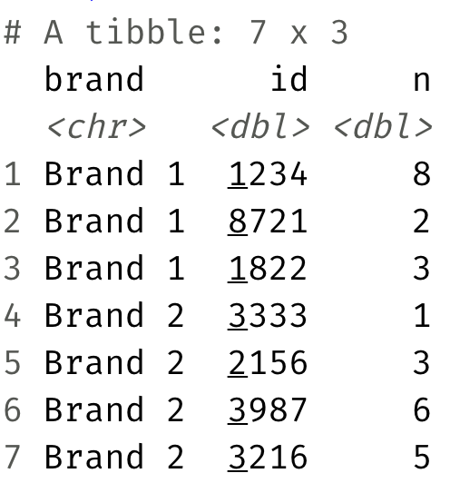
Sales data

Are these data tidy? Why or why not?

Sales data

What “data moves” do we need to go from the original, non-tidy data to this, tidy one?

ae-08-age-gaps-sales-import - Part 2

Go to your ae project in RStudio.
If you haven’t yet done so, make sure all of your changes up to this point are committed and pushed, i.e., there’s nothing left in your Git pane.
If you haven’t yet done so, click Pull to get today’s application exercise file: ae-08-age-gaps-sales-import.qmd.
Work through Part 2 of the application exercise in class, and render, commit, and push your edits.

Importing and recoding data

While you wait…

That pesky midterm…

Midterm Exam 1

In-class

Example in-class question

Example in-class question

Example in-class question

What should I put on my cheat sheet?

Take-home

Reminder: conduct policies

Things you can do to study

Let’s zoom out for a sec…

Data science and statistical thinking

Data science

Data science

From last time: data collection

Data science

From last time: data preparation

Data science

From last time: data analysis

From last time: data analysis

From last time: data analysis

From last time: data analysis

Data science

A cautionary tale: Anscombe’s quartet

A cautionary tale: Anscombe’s quartet

A cautionary tale: Anscombe’s quartet

If you only looked at summary statistics…

Our motto: ABV!

From last time

Finish up: ae-08-durham-climate-factors

Reading data into R

Reading rectangular data

Application exercise

Goal 1: Reading and writing CSV files

Age gap in Hollywood relationships

ae-08-age-gaps-sales-import - Part 1

Goal 2: Reading Excel files

Sales data

Sales data

ae-08-age-gaps-sales-import - Part 2

Finish up: `ae-08-durham-climate-factors`