Linear models with a single predictor
Lecture 13
Duke University
STA 199 Spring 2025
2025-03-04
While you wait…
Go to your
aeproject in RStudio.Make sure all of your changes up to this point are committed and pushed, i.e., there’s nothing left in your Git pane.
Click Pull to get today’s application exercise file: ae-10-modeling-penguins.qmd.
Wait till the you’re prompted to work on the application exercise during class before editing the file.
Correlation vs. causation
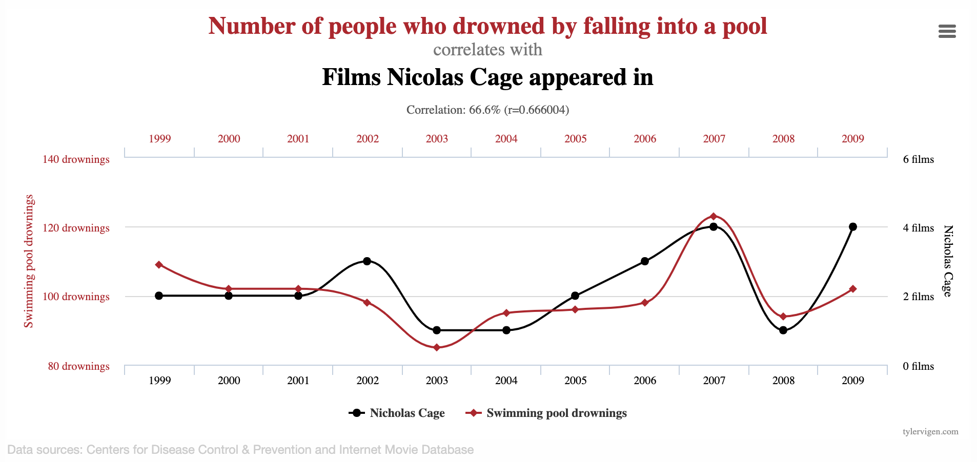
Spurious correlations

Spurious correlations
Linear regression with a single predictor
Data prep
- Rename Rotten Tomatoes columns as
criticsandaudience - Rename the dataset as
movie_scores
Data overview
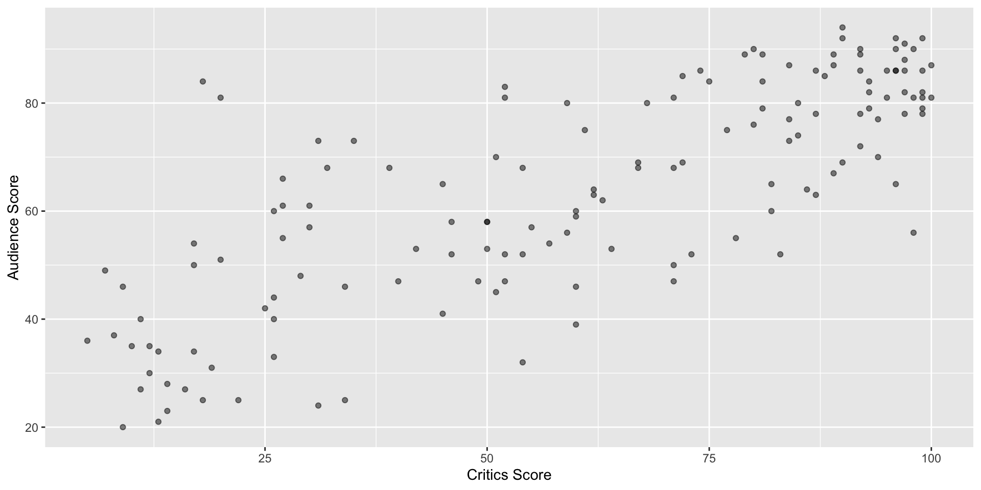
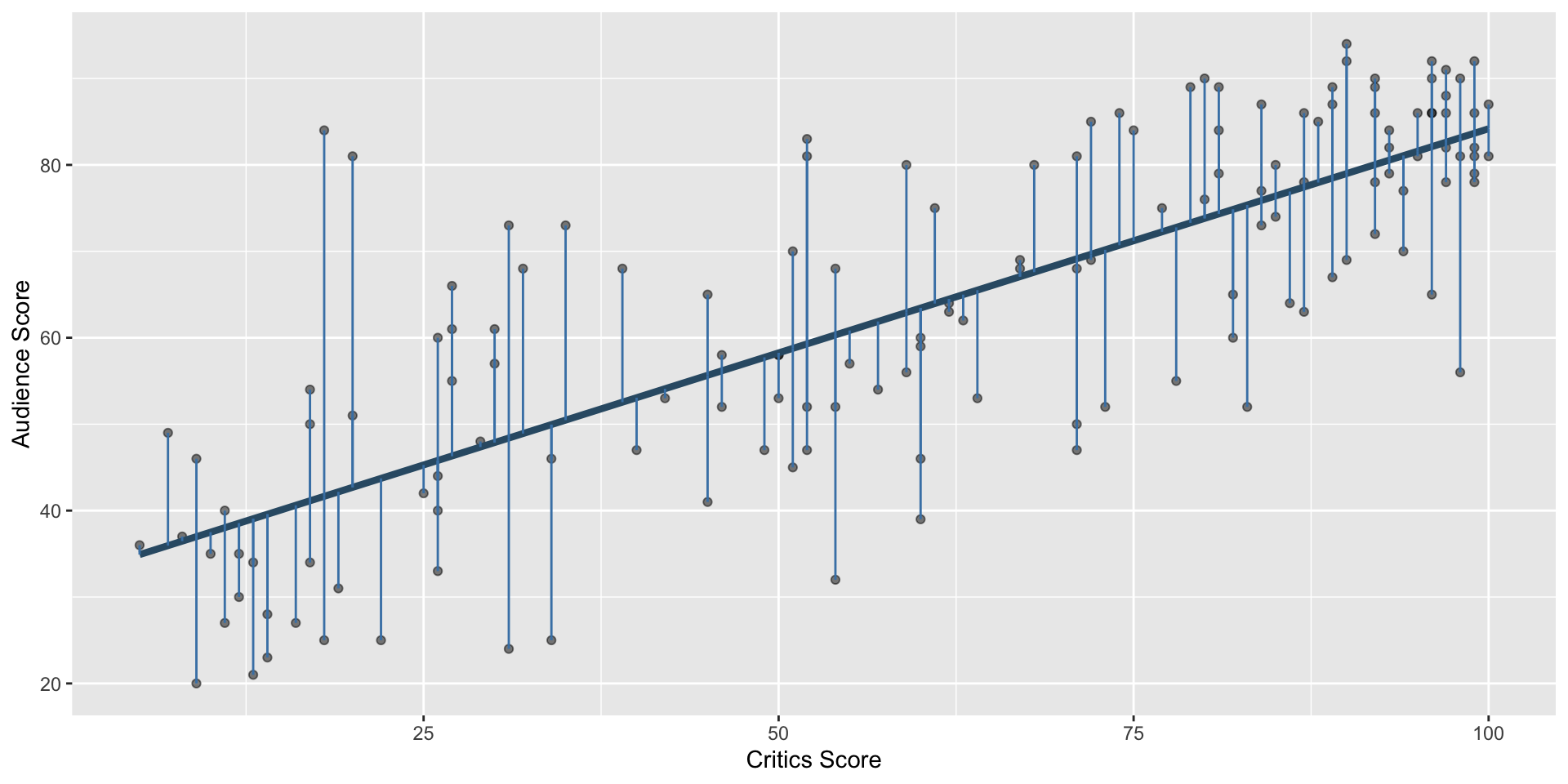
Data visualization
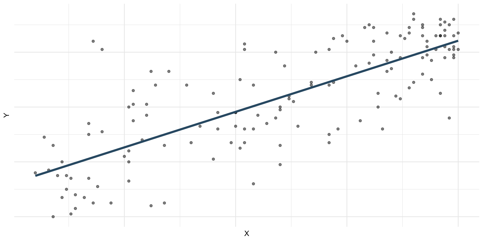
Regression model
A regression model is a function that describes the relationship between the outcome, \(Y\), and the predictor, \(X\).
\[ \begin{aligned} Y &= \color{black}{\textbf{Model}} + \text{Error} \\[8pt] &= \color{black}{\mathbf{f(X)}} + \epsilon \\[8pt] &= \color{black}{\boldsymbol{\mu_{Y|X}}} + \epsilon \end{aligned} \]
Regression model
\[ \begin{aligned} Y &= \color{#325b74}{\textbf{Model}} + \text{Error} \\[8pt] &= \color{#325b74}{\mathbf{f(X)}} + \epsilon \\[8pt] &= \color{#325b74}{\boldsymbol{\mu_{Y|X}}} + \epsilon \end{aligned} \]
Simple linear regression
Use simple linear regression to model the relationship between a quantitative outcome (\(Y\)) and a single quantitative predictor (\(X\)): \[\Large{Y = \beta_0 + \beta_1 X + \epsilon}\]
- \(\beta_1\): True slope of the relationship between \(X\) and \(Y\)
- \(\beta_0\): True intercept of the relationship between \(X\) and \(Y\)
- \(\epsilon\): Error (residual)
Simple linear regression
\[\Large{\hat{Y} = b_0 + b_1 X}\]
- \(b_1\): Estimated slope of the relationship between \(X\) and \(Y\)
- \(b_0\): Estimated intercept of the relationship between \(X\) and \(Y\)
- No error term!
Choosing values for \(b_1\) and \(b_0\)
Residuals
\[\text{residual} = \text{observed} - \text{predicted} = y - \hat{y}\]
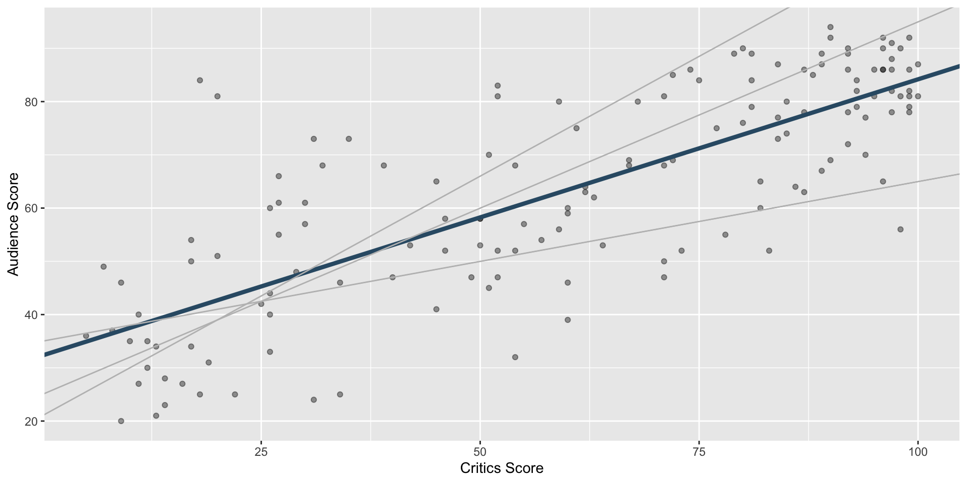
Least squares line
- The residual for the \(i^{th}\) observation is
\[e_i = \text{observed} - \text{predicted} = y_i - \hat{y}_i\]
- The sum of squared residuals is
\[e^2_1 + e^2_2 + \dots + e^2_n\]
- The least squares line is the one that minimizes the sum of squared residuals
Least squares line
Slope and intercept
Properties of least squares regression
The regression line goes through the center of mass point (the coordinates corresponding to average \(X\) and average \(Y\)): \(b_0 = \bar{Y} - b_1~\bar{X}\)
Slope has the same sign as the correlation coefficient: \(b_1 = r \frac{s_Y}{s_X}\)
Sum of the residuals is zero: \(\sum_{i = 1}^n \epsilon_i = 0\)
Residuals and \(X\) values are uncorrelated
Interpreting slope & intercept
\[\widehat{\text{audience}} = 32.3 + 0.519 \times \text{critics}\]
- Slope: For every one point increase in the critics score, we expect the audience score to be higher by 0.519 points, on average.
- Intercept: If the critics score is 0 points, we expect the audience score to be 32.3 points.
Is the intercept meaningful?
✅ The intercept is meaningful in context of the data if
- the predictor can feasibly take values equal to or near zero or
- the predictor has values near zero in the observed data
🛑 Otherwise, it might not be meaningful!
Application exercise
ae-10-modeling-penguins
Go to your ae project in RStudio.
If you haven’t yet done so, make sure all of your changes up to this point are committed and pushed, i.e., there’s nothing left in your Git pane.
If you haven’t yet done so, click Pull to get today’s application exercise file: ae-10-modeling-penguins.qmd.
Work through the application exercise in class, and render, commit, and push your edits.