Linear regression with a multiple predictors II
Lecture 15
John Zito
Duke University
STA 199 Spring 2025
2025-03-18
Quick announcements
While you wait…
Go to your
aeproject in RStudio.Make sure all of your changes up to this point are committed and pushed, i.e., there’s nothing left in your Git pane.
Click Pull to get today’s application exercise file: ae-12-modeling-loans.qmd.
Wait till the you’re prompted to work on the application exercise during class before editing the file.
Mid-semester evaluation
Please complete this ungraded, anonymous Canvas quiz before Wednesday night:
SSMU Bookbagging GBM Saturday March 22!

Grab free food and chat with upperclass students about…
- course registration
- the stats major
- DataFest
- volunteering
Project clarifications
Next Monday: your TA returns proposal feedback to you;
Until then: project repos are locked (can’t push or pull);
If you missed milestone 1, we’ll replace that score with your final peer eval score (so pull your weight!);
We will drop one of the first three peer evals;
If your group does not have plans to meet every week…make them!
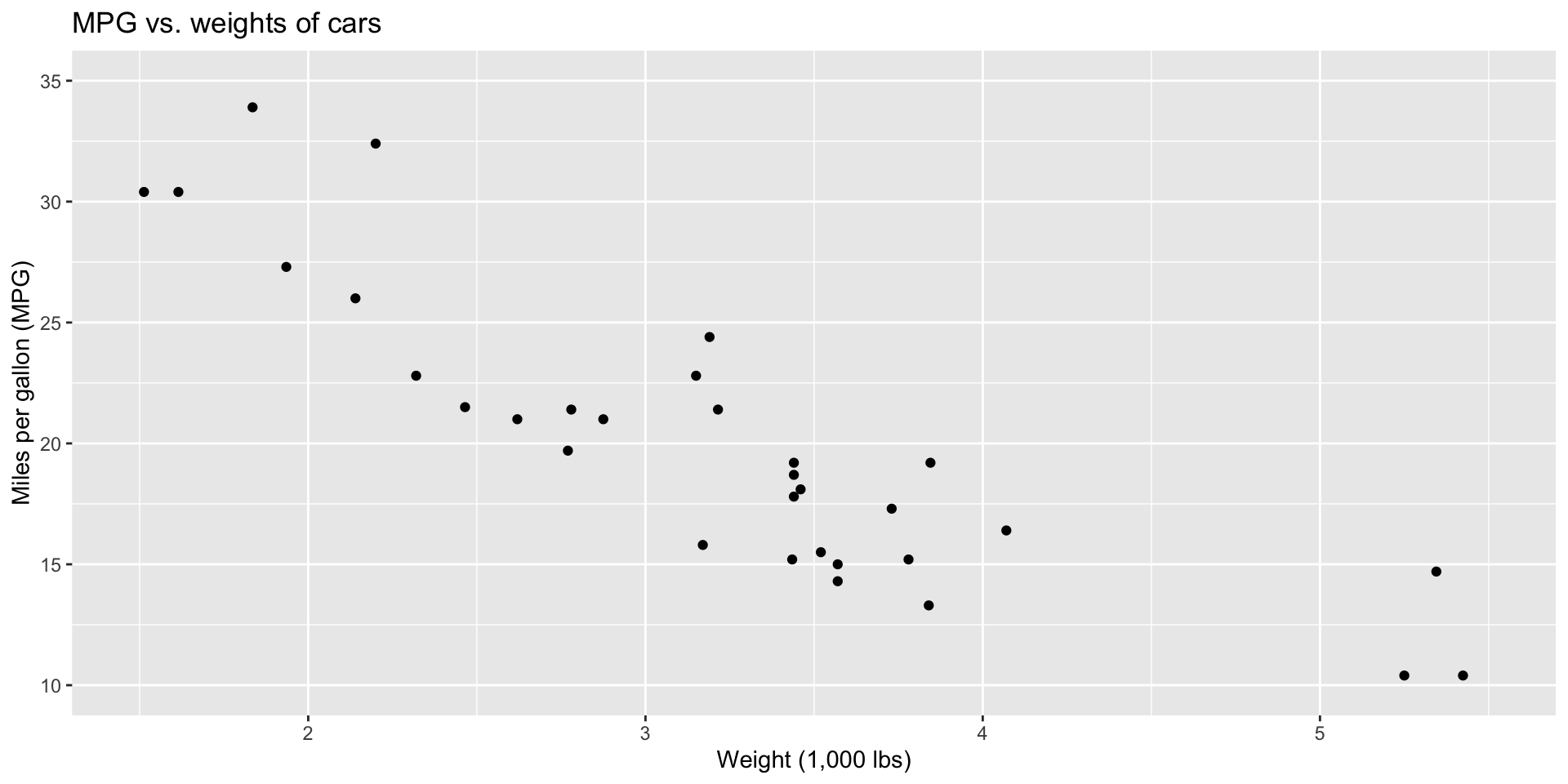
Recap: simple linear regression
Question: how do we concisely summarize the association between two variables?
Answer: simple linear regression!
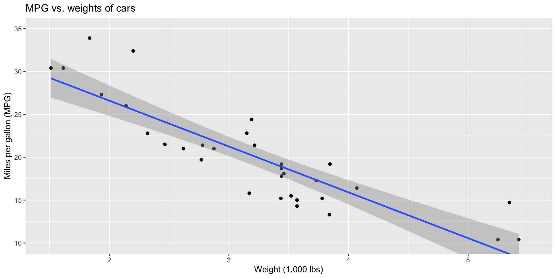
Answer: simple linear regression!
# A tibble: 2 × 5
  term        estimate std.error statistic  p.value
  <chr>          <dbl>     <dbl>     <dbl>    <dbl>
1 (Intercept)    37.3      1.88      19.9  8.24e-19
2 wt             -5.34     0.559     -9.56 1.29e-10
\[ \widehat{mpg}=37.3 - 5.34\times weight. \]
Interpretations
- We predict that a car weighing zero pounds will have 37.28 MPG on average (makes no sense);
- We predict that a 1000 pound increase in weight in associated with a 5.34 decrease in MGP, on average.
Why do we care? Prediction!
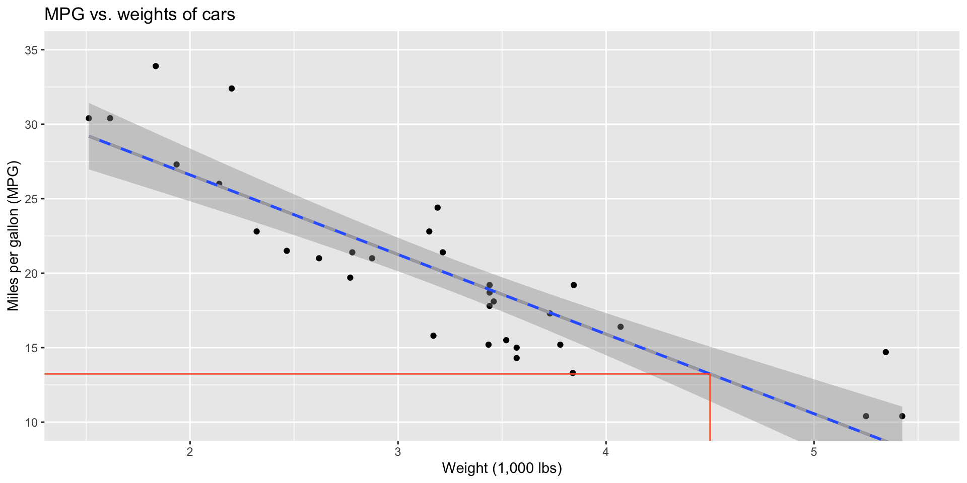
Why do we care? Prediction!
You can use the fitted model to generate predictions for yet-to-be-observed subjects:
Before break: multiple linear regression
Simple linear regression for those darn penguins
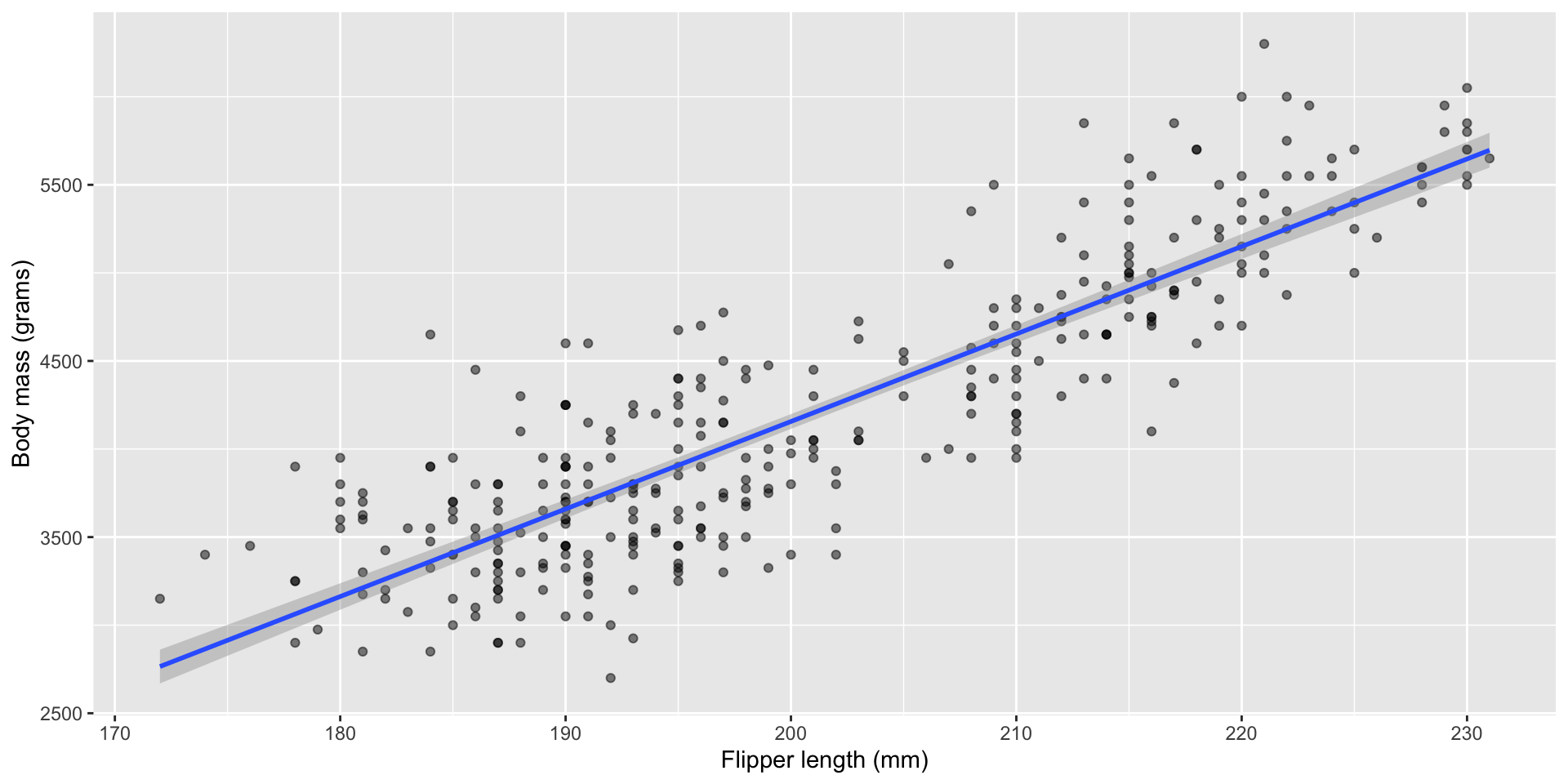
How do we predict using more than one predictor?
Both of these models use flipper_length_mm and island to predict body_mass_g:
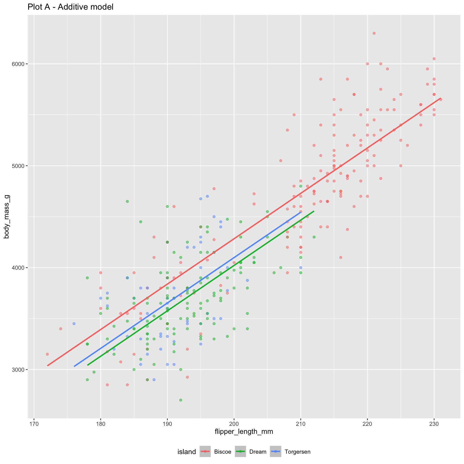
The additive model: parallel lines, one for each island
bm_fl_island_fit <- linear_reg() |>
  fit(body_mass_g ~ flipper_length_mm + island, data = penguins)

tidy(bm_fl_island_fit)
# A tibble: 4 × 5
term estimate std.error statistic p.value
<chr> <dbl> <dbl> <dbl> <dbl>
1 (Intercept) -4625. 392. -11.8 4.29e-27
2 flipper_length_mm 44.5 1.87 23.9 1.65e-74
3 islandDream -262. 55.0 -4.77 2.75e- 6
4 islandTorgersen -185. 70.3 -2.63 8.84e- 3\[ \begin{aligned} \widehat{body~mass} = -4625 &+ 44.5 \times flipper~length \\ &- 262 \times Dream \\ &- 185 \times Torgersen \end{aligned} \]
Where do the three lines come from?
\[ \begin{aligned} \widehat{body~mass} = -4625 &+ 44.5 \times flipper~length \\ &- 262 \times Dream \\ &- 185 \times Torgersen \end{aligned} \]
If penguin is from Biscoe, Dream = 0 and Torgersen = 0:
\[ \begin{aligned} \widehat{body~mass} = -4625 &+ 44.5 \times flipper~length \end{aligned} \]
If penguin is from Dream, Dream = 1 and Torgersen = 0:
\[ \begin{aligned} \widehat{body~mass} = -4887 &+ 44.5 \times flipper~length \end{aligned} \]
If penguin is from Torgersen, Dream = 0 and Torgersen = 1:
\[ \begin{aligned} \widehat{body~mass} = -4810 &+ 44.5 \times flipper~length \end{aligned} \]
Either way, same slope, so the lines are parallel.
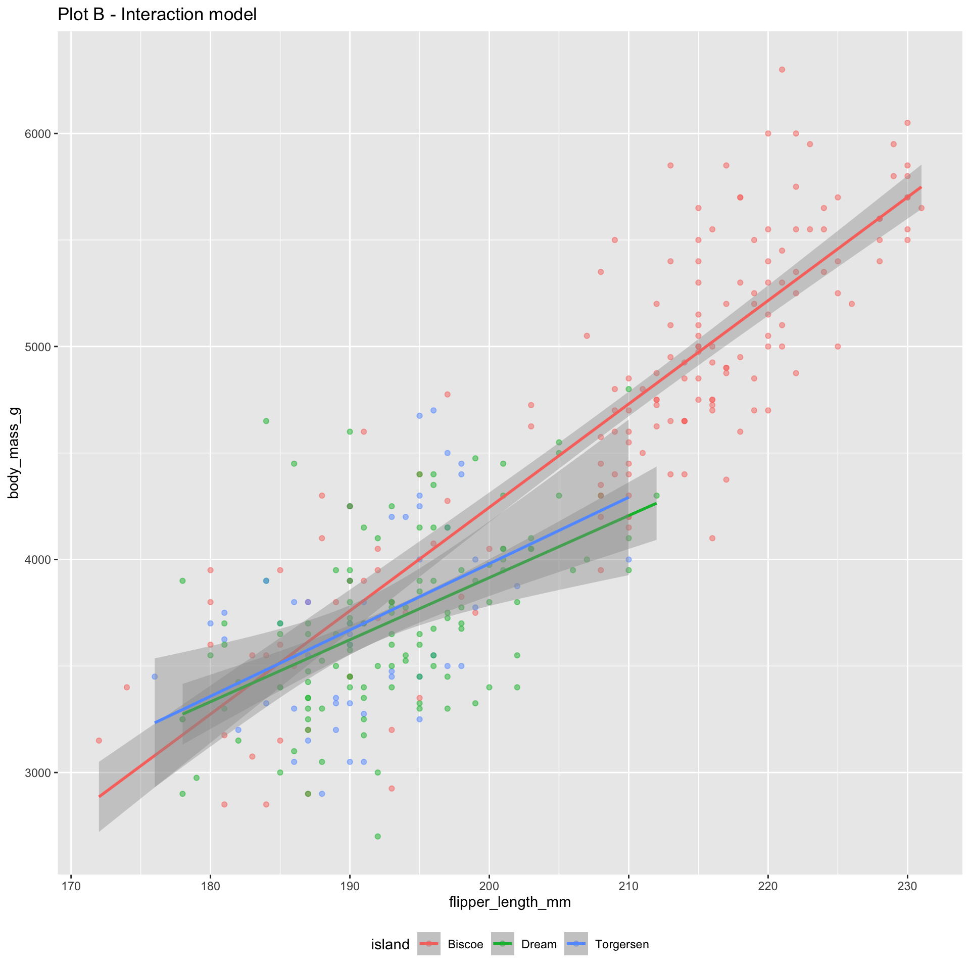
The interaction model: different lines for each island
bm_fl_island_int_fit <- linear_reg() |>
  fit(body_mass_g ~ flipper_length_mm * island, data = penguins)

tidy(bm_fl_island_int_fit) |> select(term, estimate)
# A tibble: 6 × 2
term estimate
<chr> <dbl>
1 (Intercept) -5464.
2 flipper_length_mm 48.5
3 islandDream 3551.
4 islandTorgersen 3218.
5 flipper_length_mm:islandDream -19.4
6 flipper_length_mm:islandTorgersen -17.4\[ \begin{aligned} \widehat{body~mass} = -5464 &+ 48.5 \times flipper~length \\ &+ 3551 \times Dream \\ &+ 3218 \times Torgersen \\ &- 19.4 \times flipper~length*Dream \\ &- 17.4 \times flipper~length*Torgersen \end{aligned} \]
Where do the three lines come from?
\[ \begin{aligned} \small\widehat{body~mass} = -5464 &+ 48.5 \times flipper~length \\ &+ 3551 \times Dream \\ &+ 3218 \times Torgersen \\ &- 19.4 \times flipper~length*Dream \\ &- 17.4 \times flipper~length*Torgersen \end{aligned} \]
If penguin is from Biscoe, Dream = 0 and Torgersen = 0:
\[ \begin{aligned} \widehat{body~mass} = -5464 &+ 48.5 \times flipper~length \end{aligned} \]
If penguin is from Dream, Dream = 1 and Torgersen = 0:
\[ \begin{aligned} \widehat{body~mass} &= (-5464 + 3551) + (48.5-19.4) \times flipper~length\\ &=-1913+29.1\times flipper~length. \end{aligned} \]
Prediction
new_penguin <- tibble(
  flipper_length_mm = 200,
  island = "Torgersen"
)

predict(bm_fl_island_int_fit, new_data = new_penguin)
# A tibble: 1 × 1
.pred
<dbl>
1 3980.\[ \widehat{body~mass} = (-5464 + 3218) + (48.5-17.4) \times 200. \]
Multiple numerical predictors
bm_fl_bl_fit <- linear_reg() |>
  fit(body_mass_g ~ flipper_length_mm + bill_length_mm, data = penguins)

tidy(bm_fl_bl_fit)
# A tibble: 3 × 5
term estimate std.error statistic p.value
<chr> <dbl> <dbl> <dbl> <dbl>
1 (Intercept) -5737. 308. -18.6 7.80e-54
2 flipper_length_mm 48.1 2.01 23.9 7.56e-75
3 bill_length_mm 6.05 5.18 1.17 2.44e- 1\[ \small\widehat{body~mass}=-5736+48.1\times flipper~length+6\times bill~length \]
Interpretations:
- We predict that the body mass of a penguin with zero flipper length and zero bill length will be -5736 grams, on average (makes no sense);
- Holding all other variables constant, for every additional millimeter in flipper length, we expect the body mass of penguins to be higher, on average, by 48.1 grams.
- Holding all other variables constant, for every additional millimeter in bill length, we expect the body mass of penguins to be higher, on average, by 6 grams.
Prediction
new_penguin <- tibble(
  flipper_length_mm = 200,
  bill_length_mm = 45
)

predict(bm_fl_bl_fit, new_data = new_penguin)
# A tibble: 1 × 1
.pred
<dbl>
1 4164.\[ \widehat{body~mass}=-5736+48.1\times 200+6\times 45 \]
Picture? It’s not pretty…
2 predictors + 1 response = 3 dimensions. Ick!
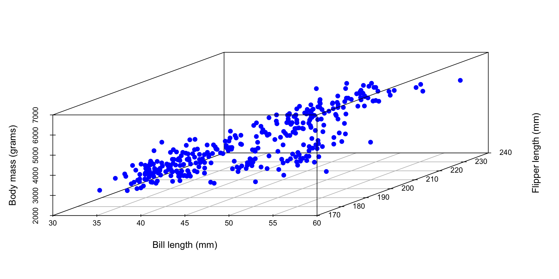
Picture? It’s not pretty…
Instead of a line of best fit, it’s a plane of best fit. Double ick!

ae-12-modeling-loans
Go to your ae project in RStudio.
If you haven’t yet done so, make sure all of your changes up to this point are committed and pushed, i.e., there’s nothing left in your Git pane.
If you haven’t yet done so, click Pull to get today’s application exercise file: ae-12-modeling-loans.qmd.
Work through the application exercise in class, and render, commit, and push your edits.