Model selection for logistic regression
Lecture 18
John Zito
Duke University
STA 199 Spring 2025
2025-03-27
While you wait…
Go to your
aeproject in RStudio.Make sure all of your changes up to this point are committed and pushed, i.e., there’s nothing left in your Git pane.
Click Pull to get today’s application exercise file: ae-14-forest-classification.qmd.
Wait till the you’re prompted to work on the application exercise during class before editing the file.
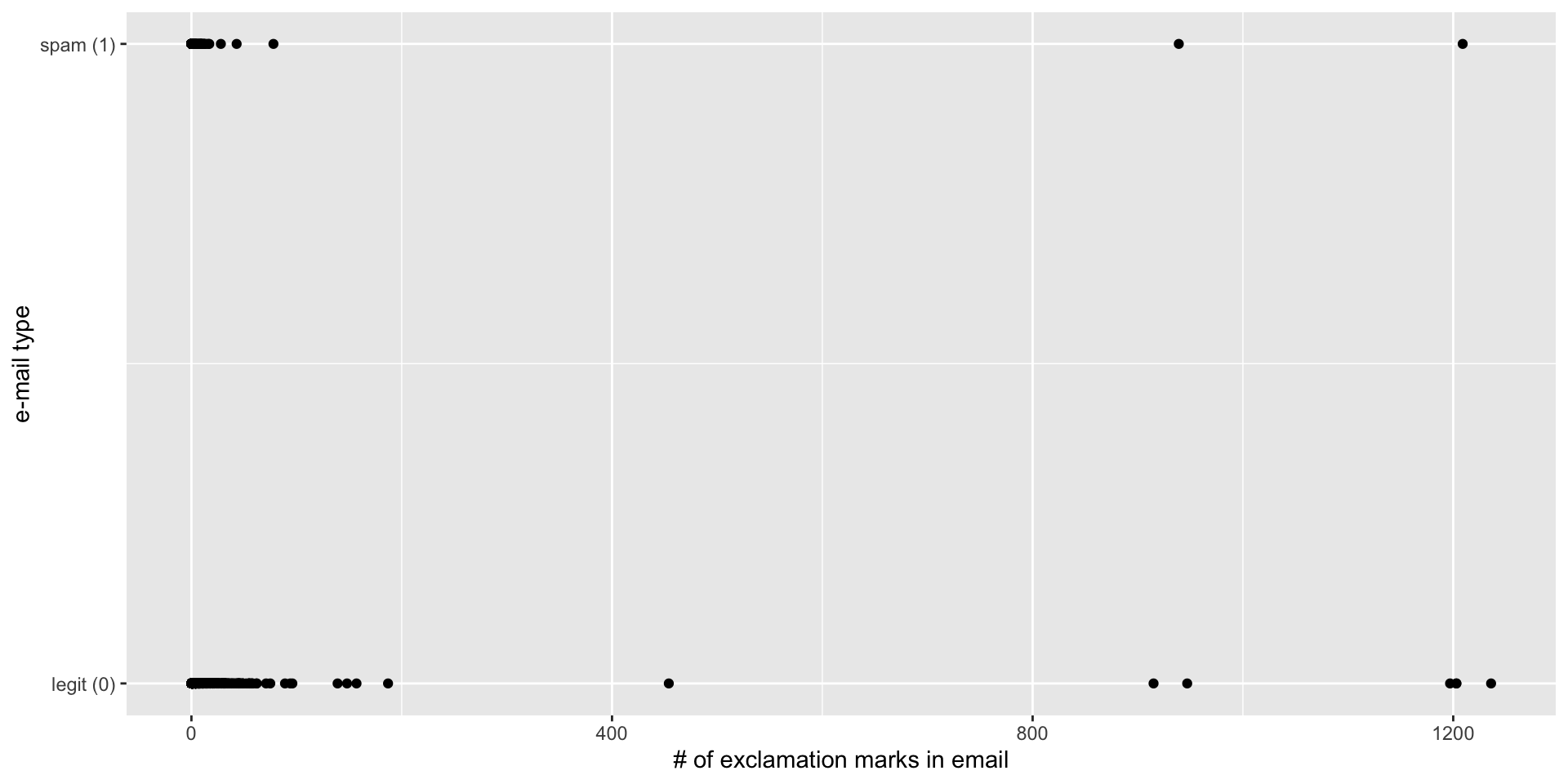
Last time: regression with a binary response
New model: logistic regression
S-curve for the probability of success \(p=P(y=1)\):
\[ \hat{p} = \frac{e^{b_0+b_1x}}{1+e^{b_0+b_1x}}. \]
Linear model for the log-odds:
\[ \log\left(\frac{\hat{p}}{1-\hat{p}}\right) = b_0+b_1x. \]
These are equivalent.
R syntax is mostly unchanged
simple_logistic_fit <- logistic_reg() |>
  fit(spam ~ exclaim_mess, data = email)

tidy(simple_logistic_fit)
# A tibble: 2 × 5
term estimate std.error statistic p.value
<chr> <dbl> <dbl> <dbl> <dbl>
1 (Intercept) -2.27 0.0553 -41.1 0
2 exclaim_mess 0.000272 0.000949 0.287 0.774Fitted equation for the log-odds:
\[ \log\left(\frac{\hat{p}}{1-\hat{p}}\right) = -2.27 + 0.000272\times exclaim~mess \]
Interpretations are strange and delicate.
Here’s an alternative model
Dump all the predictors in:
# A tibble: 22 × 5
   term         estimate std.error statistic  p.value
   <chr>           <dbl>     <dbl>     <dbl>    <dbl>
 1 (Intercept)  -9.09e+1   9.80e+3  -0.00928 9.93e- 1
 2 to_multiple1 -2.68e+0   3.27e-1  -8.21    2.25e-16
 3 from1        -2.19e+1   9.80e+3  -0.00224 9.98e- 1
 4 cc            1.88e-2   2.20e-2   0.855   3.93e- 1
 5 sent_email1  -2.07e+1   3.87e+2  -0.0536  9.57e- 1
 6 time          8.48e-8   2.85e-8   2.98    2.92e- 3
 7 image        -1.78e+0   5.95e-1  -3.00    2.73e- 3
 8 attach        7.35e-1   1.44e-1   5.09    3.61e- 7
 9 dollar       -6.85e-2   2.64e-2  -2.59    9.64e- 3
10 winneryes     2.07e+0   3.65e-1   5.67    1.41e- 8
# ℹ 12 more rows
Classification error
There are two kinds of mistakes:
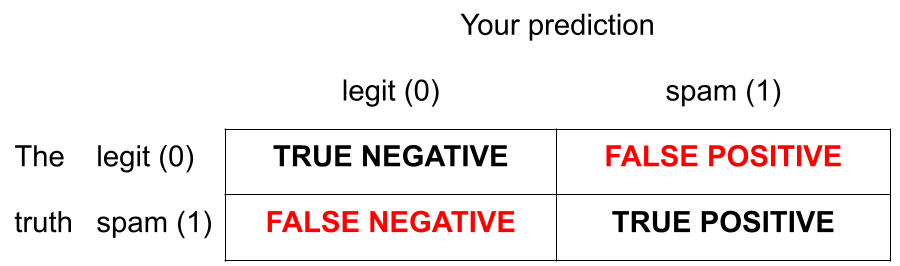
We want to avoid both, but there’s a trade-off.
Jargon: False negative and positive
False negative rate is the proportion of actual positives that were classified as negatives.
False positive rate is the proportion of actual negatives that were classified as positives.
Tip
We want these to be low!
Jargon: Sensitivity
Sensitivity is the proportion of actual positives that were correctly classified as positive.
Also known as true positive rate and recall
Sensitivity = 1 − False negative rate
Useful when false negatives are more “expensive” than false positives
Tip
We want this to be high!
Jargon: Specificity
Specificity is the proportion of actual negatives that were correctly classified as negative
Also known as true negative rate
Specificity = 1 − False positive rate
Tip
We want this to be high!
The augment function
The augment function takes a data frame and “augments” it by adding three new columns on the left that describe the model predictions for each row:
-
.pred_class: model prediction (\(\hat{y}\)) based on a 50% threshold; -
.pred_0: model estimate of \(P(y=0)\); -
.pred_1: model estimate of \(P(y=1) = 1 - P(y = 0)\).
The augment function
The augment function takes a data frame and “augments” it by adding three new columns on the left that describe the model predictions for each row:
# A tibble: 3,921 × 24
   .pred_class .pred_0  .pred_1 spam  to_multiple from     cc sent_email
   <fct>         <dbl>    <dbl> <fct> <fct>       <fct> <int> <fct>
 1 0             0.867 1.33e- 1 0     0           1         0 0
 2 0             0.943 5.70e- 2 0     0           1         0 0
 3 0             0.942 5.78e- 2 0     0           1         0 0
 4 0             0.920 7.96e- 2 0     0           1         0 0
 5 0             0.903 9.74e- 2 0     0           1         0 0
 6 0             0.901 9.87e- 2 0     0           1         0 0
 7 0             1.000 7.89e-12 0     1           1         0 1
 8 0             1.000 1.24e-12 0     1           1         1 1
 9 0             0.862 1.38e- 1 0     0           1         0 0
10 0             0.922 7.76e- 2 0     0           1         0 0
# ℹ 3,911 more rows
# ℹ 16 more variables: time <dttm>, image <dbl>, attach <dbl>, dollar <dbl>,
#   winner <fct>, inherit <dbl>, viagra <dbl>, password <dbl>, num_char <dbl>,
#   line_breaks <int>, format <fct>, re_subj <fct>, exclaim_subj <dbl>,
#   urgent_subj <fct>, exclaim_mess <dbl>, number <fct>
Calculating the error rates
Calculating the error rates
Calculating the error rates
Calculating the error rates
log_aug_full |>
count(spam, .pred_class) |>
group_by(spam) |>
mutate(
p = n / sum(n),
decision = case_when(
spam == "0" & .pred_class == "0" ~ "True negative",
spam == "0" & .pred_class == "1" ~ "False positive",
spam == "1" & .pred_class == "0" ~ "False negative",
spam == "1" & .pred_class == "1" ~ "True positive"
))# A tibble: 4 × 5
# Groups: spam [2]
spam .pred_class n p decision
<fct> <fct> <int> <dbl> <chr>
1 0 0 3521 0.991 True negative
2 0 1 33 0.00929 False positive
3 1 0 299 0.815 False negative
4 1 1 68 0.185 True positive But wait!
If we change the classification threshold, we change the classifications, and we change the error rates:
Classification threshold: 0.00
Classification threshold: 0.25
Classification threshold: 0.5
Classification threshold: 0.75
Classification threshold: 1.00
Let’s plot these error rates
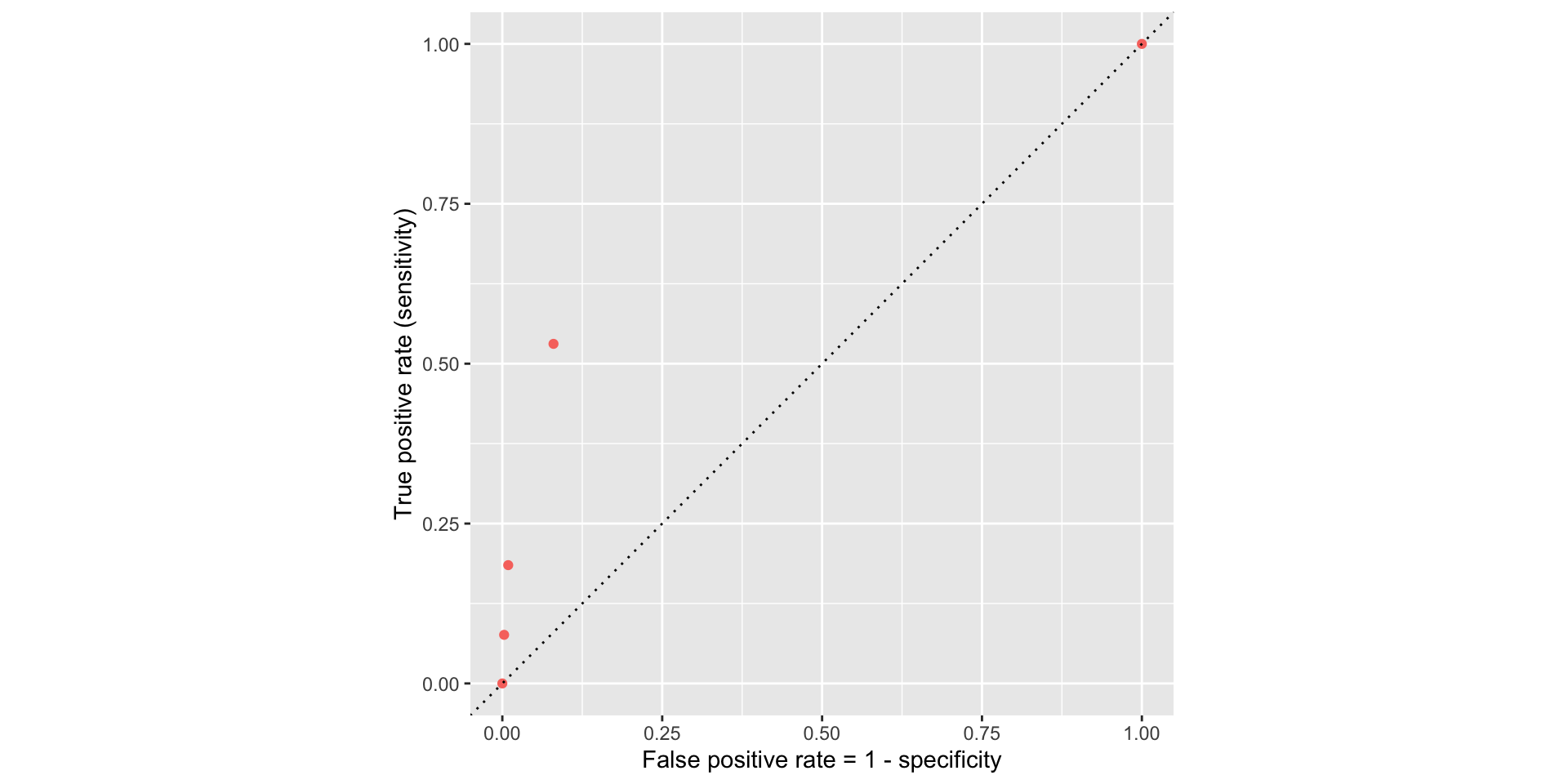
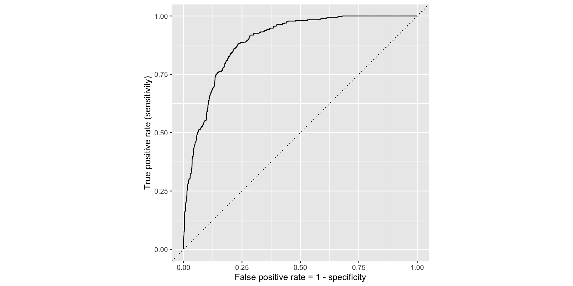
ROC curve
If we repeat this process for “all” possible thresholds \(0\leq p^\star\leq 1\), we trace out the receiver operating characteristic curve (ROC curve), which assesses the model’s performance across a range of thresholds:

ROC curve
Which corner of the plot indicates the best model performance?
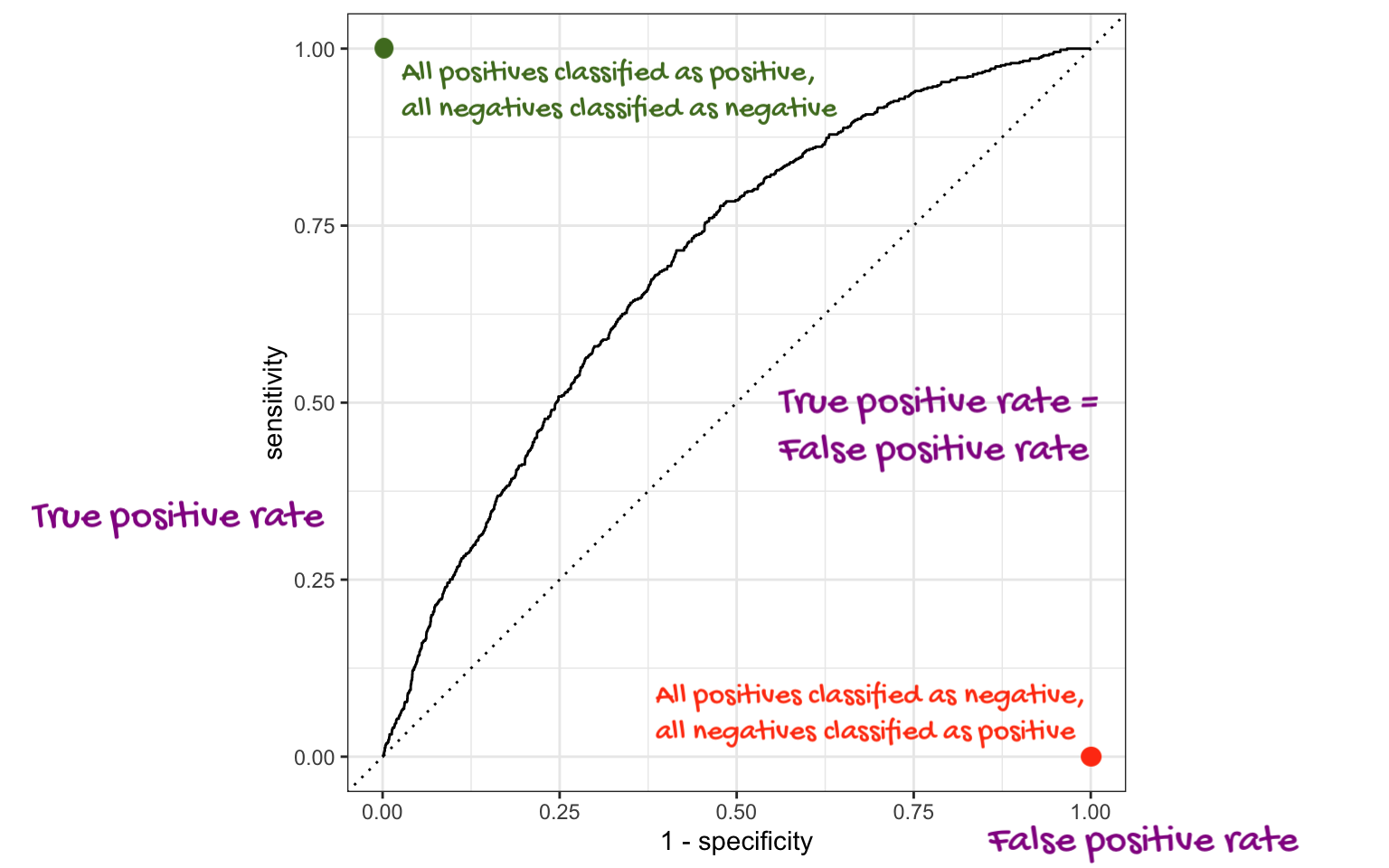
Upper left!
ROC for full model

ROC for simple model
Comparing these two curves, the full model is better.
Model comparison
The farther up and to the left the ROC curve is, the better the classification accuracy. You can quantify this with the area under the curve.
Note
Area under the ROC curve will be our “quality score” for comparing logistic regression models.
Washington forests
Data
The U.S. Forest Service maintains machine learning models to predict whether a plot of land is “forested.”
This classification is important for research, legislation, land management, etc. purposes.
Plots are typically remeasured every 10 years.
The
foresteddataset contains the most recent measurement per plot.
Data: forested
# A tibble: 7,107 × 20
   forested  year elevation eastness northness roughness tree_no_tree dew_temp
   <fct>    <dbl>     <dbl>    <dbl>     <dbl>     <dbl> <fct>           <dbl>
 1 Yes       2005       881       90        43        63 Tree             0.04
 2 Yes       2005       113      -25        96        30 Tree             6.4
 3 No        2005       164      -84        53        13 Tree             6.06
 4 Yes       2005       299       93        34         6 No tree          4.43
 5 Yes       2005       806       47       -88        35 Tree             1.06
 6 Yes       2005       736      -27       -96        53 Tree             1.35
 7 Yes       2005       636      -48        87         3 No tree          1.42
 8 Yes       2005       224      -65       -75         9 Tree             6.39
 9 Yes       2005        52      -62        78        42 Tree             6.5
10 Yes       2005      2240      -67       -74        99 No tree         -5.63
# ℹ 7,097 more rows
# ℹ 12 more variables: precip_annual <dbl>, temp_annual_mean <dbl>,
#   temp_annual_min <dbl>, temp_annual_max <dbl>, temp_january_min <dbl>,
#   vapor_min <dbl>, vapor_max <dbl>, canopy_cover <dbl>, lon <dbl>, lat <dbl>,
#   land_type <fct>, county <fct>
Data: forested
Rows: 7,107
Columns: 20
$ forested         <fct> Yes, Yes, No, Yes, Yes, Yes, Yes, Yes, Yes, Yes, Yes,…
$ year             <dbl> 2005, 2005, 2005, 2005, 2005, 2005, 2005, 2005, 2005,…
$ elevation        <dbl> 881, 113, 164, 299, 806, 736, 636, 224, 52, 2240, 104…
$ eastness         <dbl> 90, -25, -84, 93, 47, -27, -48, -65, -62, -67, 96, -4…
$ northness        <dbl> 43, 96, 53, 34, -88, -96, 87, -75, 78, -74, -26, 86, …
$ roughness        <dbl> 63, 30, 13, 6, 35, 53, 3, 9, 42, 99, 51, 190, 95, 212…
$ tree_no_tree     <fct> Tree, Tree, Tree, No tree, Tree, Tree, No tree, Tree,…
$ dew_temp         <dbl> 0.04, 6.40, 6.06, 4.43, 1.06, 1.35, 1.42, 6.39, 6.50,…
$ precip_annual    <dbl> 466, 1710, 1297, 2545, 609, 539, 702, 1195, 1312, 103…
$ temp_annual_mean <dbl> 6.42, 10.64, 10.07, 9.86, 7.72, 7.89, 7.61, 10.45, 10…
$ temp_annual_min  <dbl> -8.32, 1.40, 0.19, -1.20, -5.98, -6.00, -5.76, 1.11, …
$ temp_annual_max  <dbl> 12.91, 15.84, 14.42, 15.78, 13.84, 14.66, 14.23, 15.3…
$ temp_january_min <dbl> -0.08, 5.44, 5.72, 3.95, 1.60, 1.12, 0.99, 5.54, 6.20…
$ vapor_min        <dbl> 78, 34, 49, 67, 114, 67, 67, 31, 60, 79, 172, 162, 70…
$ vapor_max        <dbl> 1194, 938, 754, 1164, 1254, 1331, 1275, 944, 892, 549…
$ canopy_cover     <dbl> 50, 79, 47, 42, 59, 36, 14, 27, 82, 12, 74, 66, 83, 6…
$ lon              <dbl> -118.6865, -123.0825, -122.3468, -121.9144, -117.8841…
$ lat              <dbl> 48.69537, 47.07991, 48.77132, 45.80776, 48.07396, 48.…
$ land_type        <fct> Tree, Tree, Tree, Tree, Tree, Tree, Non-tree vegetati…
$ county           <fct> Ferry, Thurston, Whatcom, Skamania, Stevens, Stevens,…
Outcome and predictors
- Outcome:
forested- Factor,YesorNo
-
Predictors: 18 remotely-sensed and easily-accessible predictors:
numeric variables based on weather and topography
categorical variables based on classifications from other governmental organizations
?forested
Should we include a predictor?
To determine whether we should include a predictor in a model, we should start by asking:
Is it ethical to use this variable? (Or even legal?)
Will this variable be available at prediction time?
Does this variable contribute to explainability?
Data splitting and spending
We’ve been cheating!
So far, we’ve been using all the data we have for building models. In predictive contexts, this would be considered cheating.
Evaluating model performance for predicting outcomes that were used when building the models is like evaluating your learning with questions whose answers you’ve already seen.
Spending your data
For predictive models (used primarily in machine learning), we typically split data into training and test sets:

The training set is used to estimate model parameters.
The test set is used to find an independent assessment of model performance.
Warning
Do not use, or even peek at, the test set during training.
How much to spend?
The more data we spend (use in training), the better estimates we’ll get.
Spending too much data in training prevents us from computing a good assessment of predictive performance.
Spending too much data in testing prevents us from computing a good estimate of model parameters.
The initial split
Setting a seed
What does set.seed() do?
To create that split of the data, R generates “pseudo-random” numbers: while they are made to behave like random numbers, their generation is deterministic given a “seed”.
This allows us to reproduce results by setting that seed.
Which seed you pick doesn’t matter, as long as you don’t try a bunch of seeds and pick the one that gives you the best performance.
Accessing the data
The training set
# A tibble: 5,330 × 20
   forested  year elevation eastness northness roughness tree_no_tree dew_temp
   <fct>    <dbl>     <dbl>    <dbl>     <dbl>     <dbl> <fct>           <dbl>
 1 Yes       2013       315      -17        98        92 Tree             5.83
 2 No        2018       374       93       -34        23 No tree          0.7
 3 No        2017       377       44       -89         1 Tree             1.83
 4 Yes       2013       541       31       -94       139 Tree             4.19
 5 Yes       2017       680       14       -98        20 Tree             0.79
 6 Yes       2017      1482       76       -64        43 Tree            -0.18
 7 No        2020        84       42       -90        12 No tree          6.9
 8 Yes       2011       210       34        93        16 Tree             5.52
 9 No        2020       766       14        98        20 No tree          1.52
10 Yes       2013      1559       98        16        79 Tree            -3.45
# ℹ 5,320 more rows
# ℹ 12 more variables: precip_annual <dbl>, temp_annual_mean <dbl>,
#   temp_annual_min <dbl>, temp_annual_max <dbl>, temp_january_min <dbl>,
#   vapor_min <dbl>, vapor_max <dbl>, canopy_cover <dbl>, lon <dbl>, lat <dbl>,
#   land_type <fct>, county <fct>
The testing data
# A tibble: 1,777 × 20
   forested  year elevation eastness northness roughness tree_no_tree dew_temp
   <fct>    <dbl>     <dbl>    <dbl>     <dbl>     <dbl> <fct>           <dbl>
 1 Yes       2005       881       90        43        63 Tree             0.04
 2 Yes       2005       636      -48        87         3 No tree          1.42
 3 Yes       2005      2240      -67       -74        99 No tree         -5.63
 4 Yes       2014       940      -93        35        50 Tree            -0.15
 5 No        2014       246       22       -97         5 Tree             2.41
 6 No        2014       419       86       -49         5 No tree          1.87
 7 No        2014       308      -70       -70         4 No tree          3.07
 8 No        2014       302      -31       -94         1 No tree          2.55
 9 No        2014       340      -54        83        60 No tree          1.29
10 No        2014       792      -61       -79        30 No tree          0.25
# ℹ 1,767 more rows
# ℹ 12 more variables: precip_annual <dbl>, temp_annual_mean <dbl>,
#   temp_annual_min <dbl>, temp_annual_max <dbl>, temp_january_min <dbl>,
#   vapor_min <dbl>, vapor_max <dbl>, canopy_cover <dbl>, lon <dbl>, lat <dbl>,
#   land_type <fct>, county <fct>
Exploratory data analysis
Initial questions
What’s the distribution of the outcome,
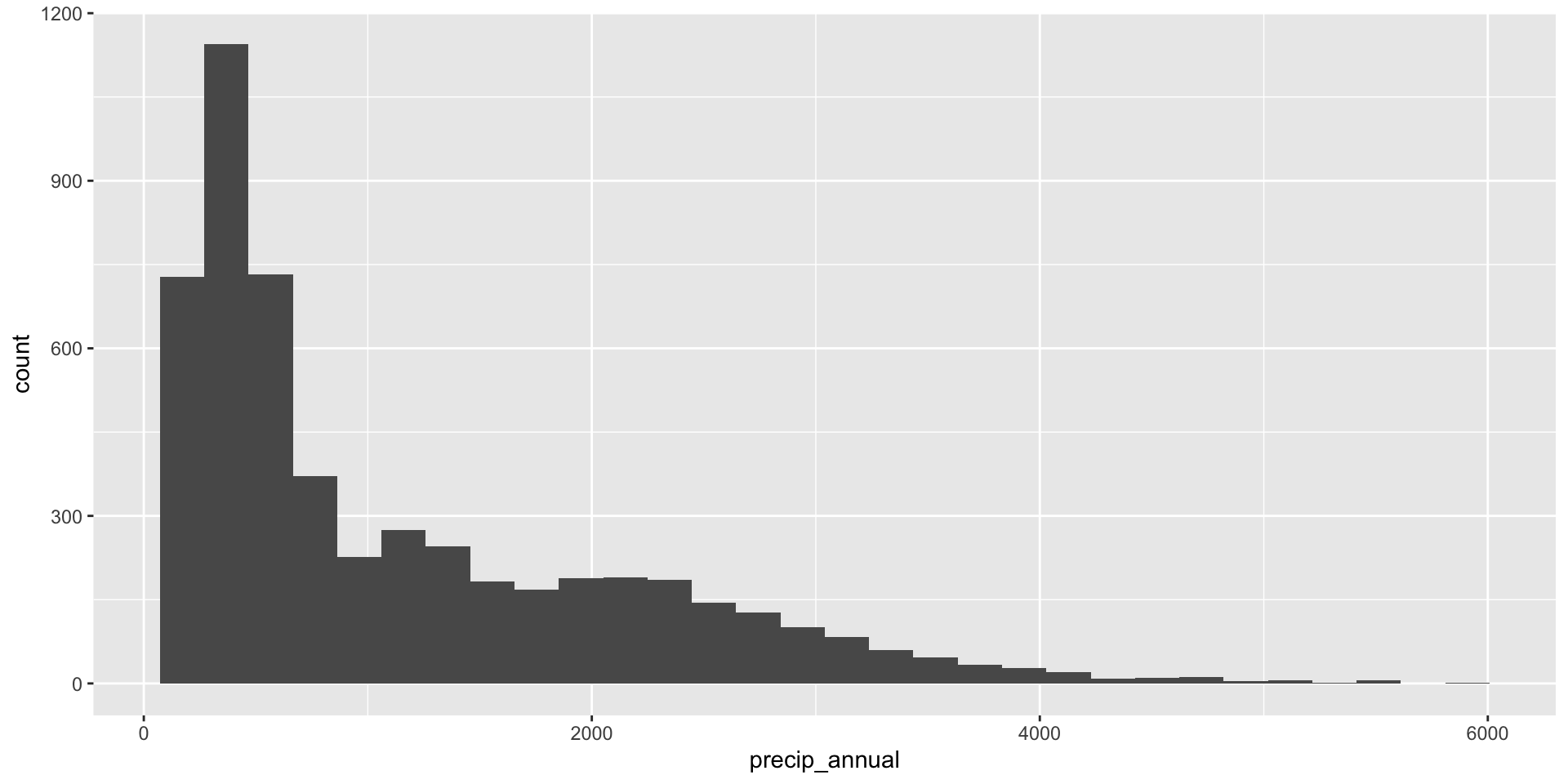
forested?What’s the distribution of numeric variables like
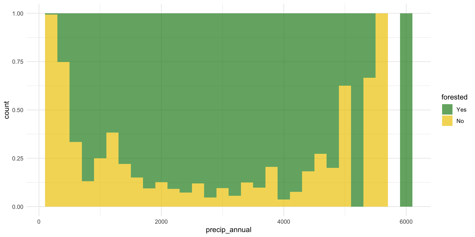
precip_annual?How does the distribution of forested differ across the categorical and numerical variables?
Which dataset should we use for the exploration? The entire data forested, the training data forested_train, or the testing data forested_test?
forested
What’s the distribution of the outcome, forested?
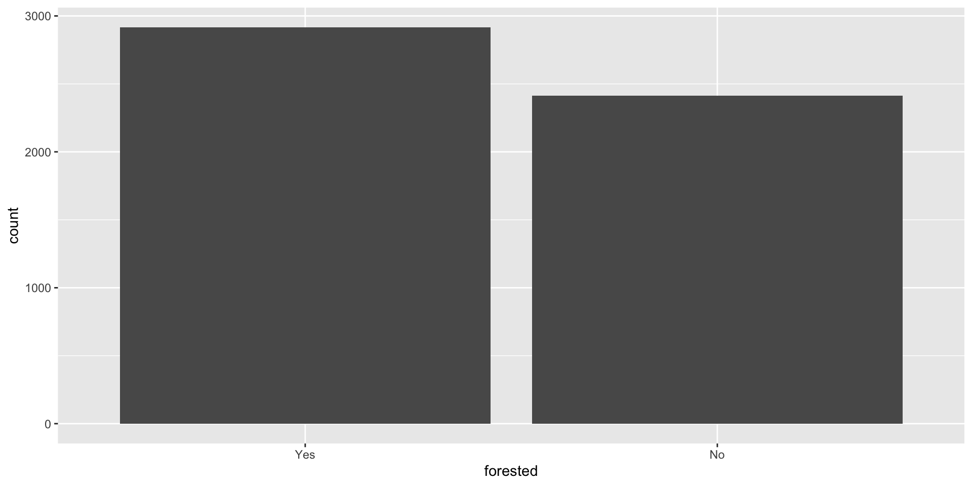
forested
What’s the distribution of the outcome, forested?
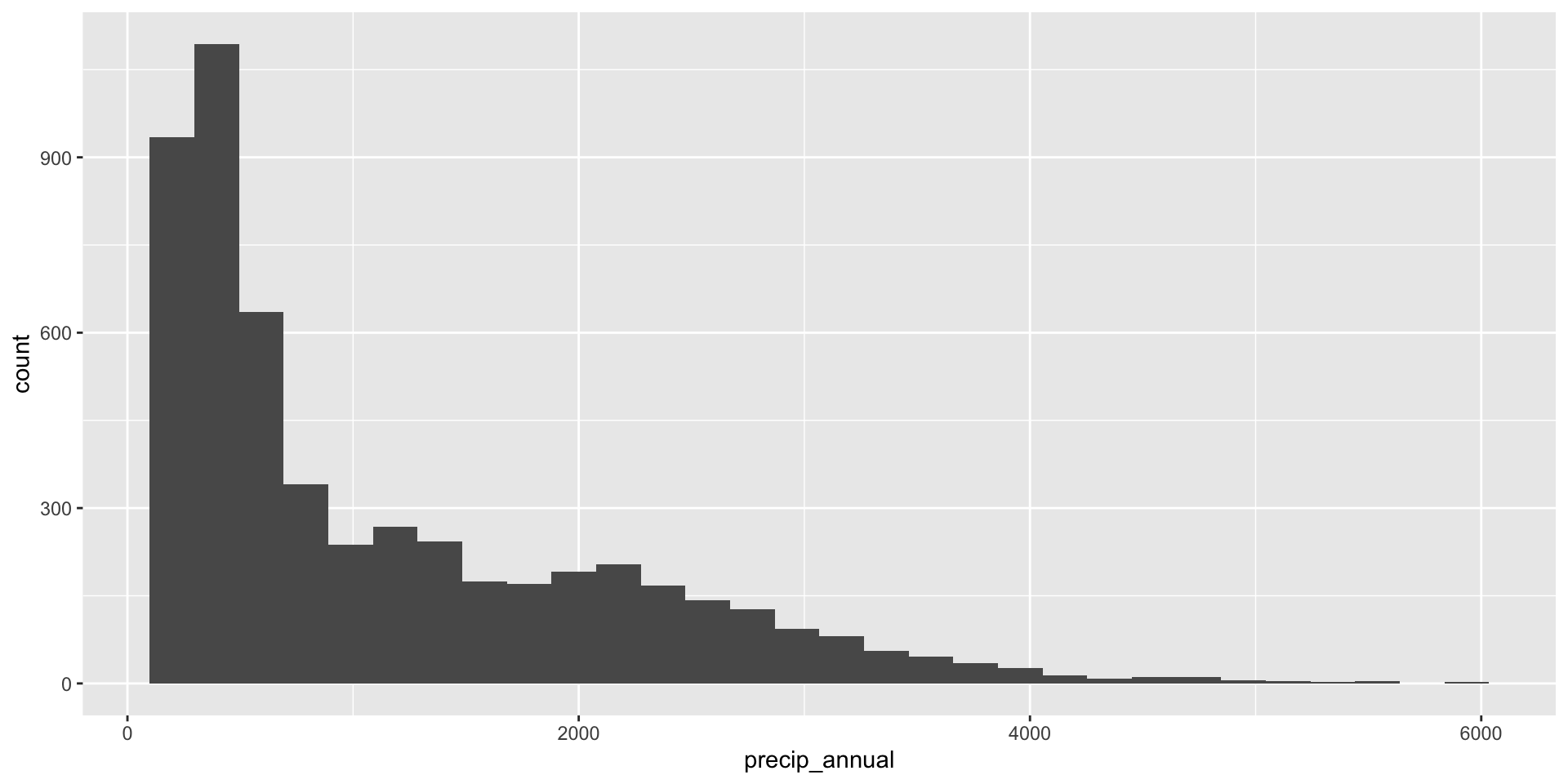
precip_annual
What’s the distribution of precip_annual?
forested and precip_annual

forested and precip_annual
forested and tree_no_tree
forested and lat / lon

Next steps
Next steps
Fit models on training data
Make predictions on testing data
-
Evaluate predictions on testing data:
- Linear models: R-squared, adjusted R-squared, RMSE (root mean squared error), etc.
- Logistic models: False negative and positive rates, AUC (area under the curve), etc.
Make decisions based on model predictive performance, validity across various testing/training splits (aka “cross validation”), explainability
Note
We will only learn about a subset of these in this course, but you can go further into these ideas in STA 210 or STA 221 as well as in various machine learning courses.
ae-14-forest-classification
Go to your ae project in RStudio.
If you haven’t yet done so, make sure all of your changes up to this point are committed and pushed, i.e., there’s nothing left in your Git pane.
If you haven’t yet done so, click Pull to get today’s application exercise file: ae-14-forest-classification.qmd. You might be prompted to install forested, say yes.
Work through the application exercise in class, and render, commit, and push your edits.