Hypothesis testing

Lecture 20

John Zito

Duke University
STA 199 Spring 2025

2025-04-03

While you wait…

• Go to your ae project in RStudio.

• Make sure all of your changes up to this point are committed and pushed, i.e., there’s nothing left in your Git pane.

• Click Pull to get today’s application exercise file: ae-16-hypothesis-testing.qmd.

• Wait till the you’re prompted to work on the application exercise during class before editing the file.

Midterm 2

• Practice: released tonight or tomorrow;

  • Solutions posted next Monday;
  • Lab 7 solutions posted next Tuesday night;

• Review: Kahoot during lab Monday April 7;

• In-class: Thursday April 10 at 11:45 AM;

  • Expect an email from Dr. Knox about room assignments;

• Take-home: 4/10 1:00 PM - 4/14 8:30 AM;

• Expect similar style, format, and intensity as Midterm 1;

• Statistical inference will appear!

Recap: sampling uncertainty

What if this was my dataset?

# A tibble: 2 × 2
  term        estimate
  <chr>          <dbl>
1 (Intercept)    2.94 
2 log_inc        0.657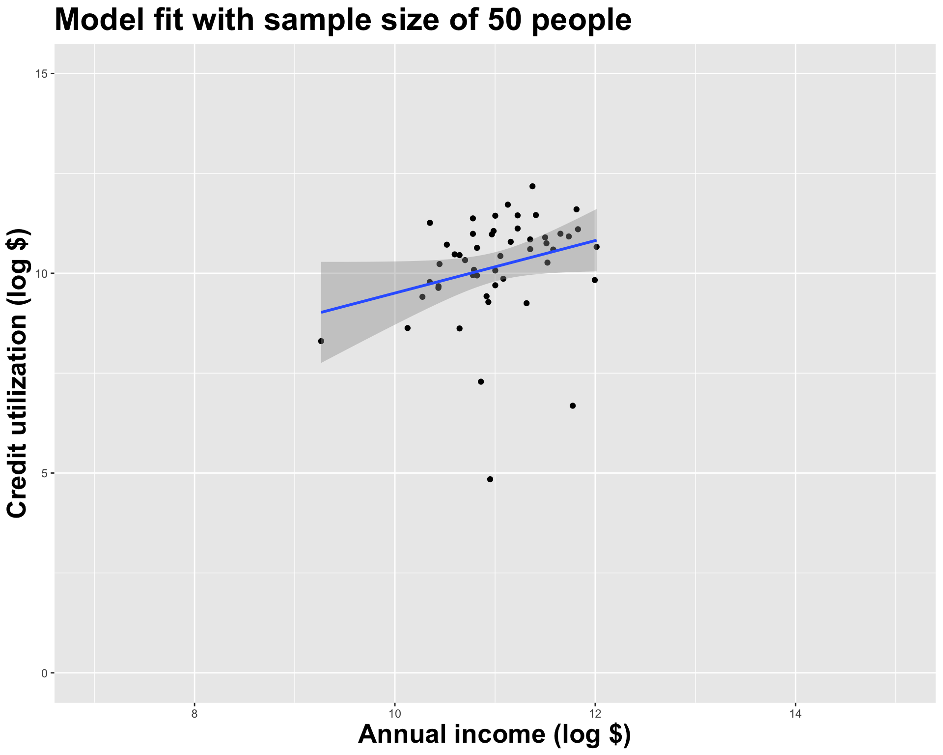

What if this was my dataset instead?

# A tibble: 2 × 2
  term        estimate
  <chr>          <dbl>
1 (Intercept)    5.29 
2 log_inc        0.486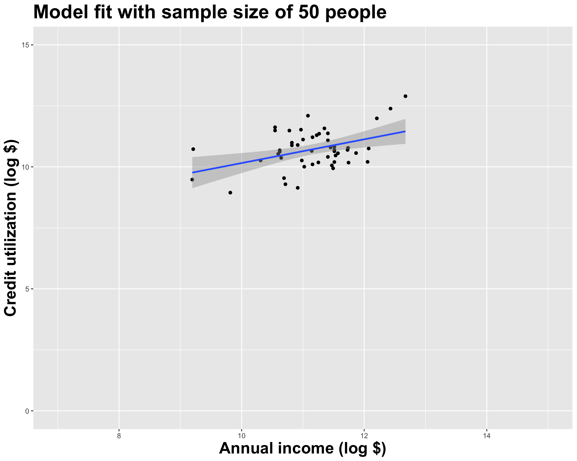

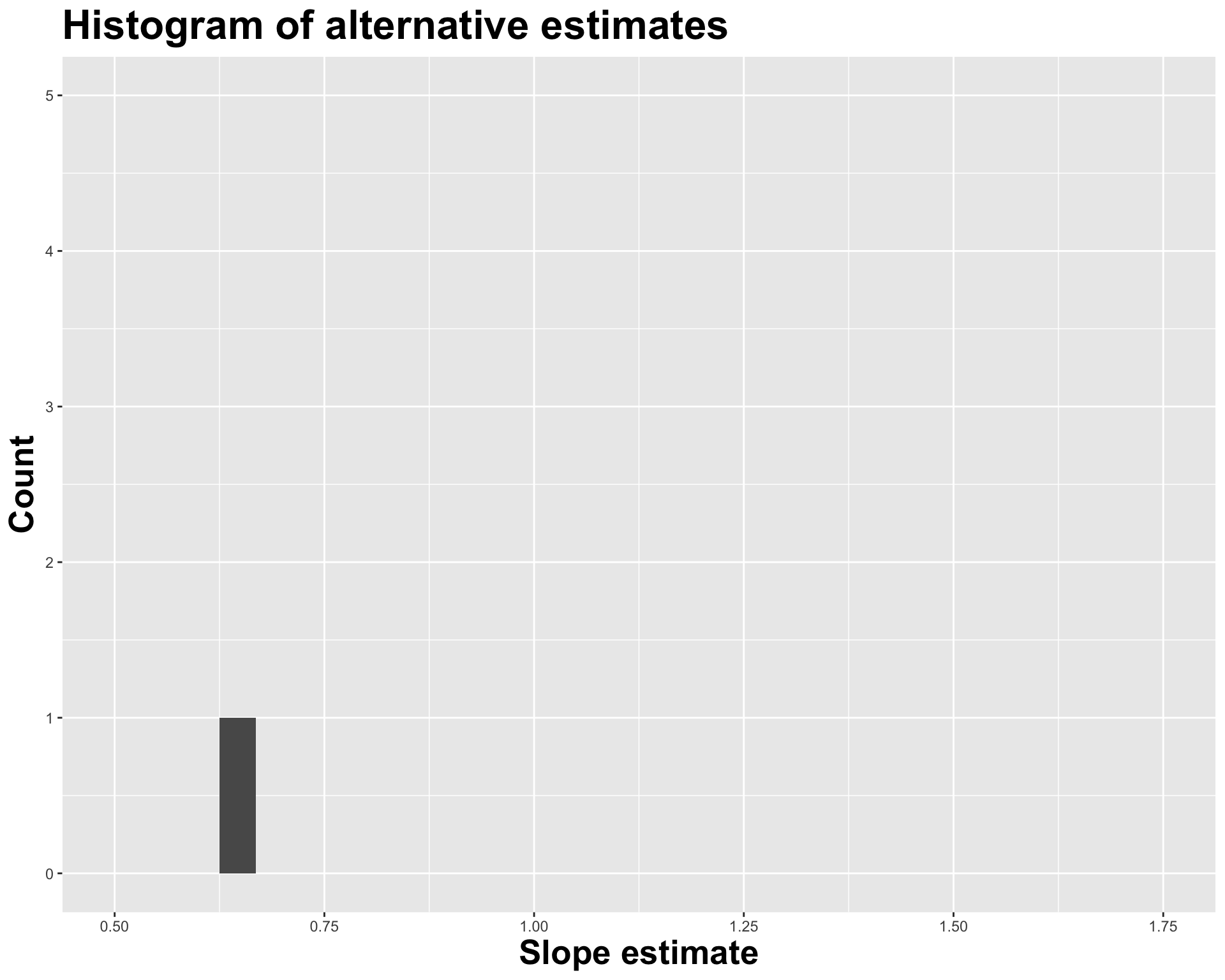
What if this was my dataset instead?

# A tibble: 2 × 2
  term        estimate
  <chr>          <dbl>
1 (Intercept)    1.62 
2 log_inc        0.805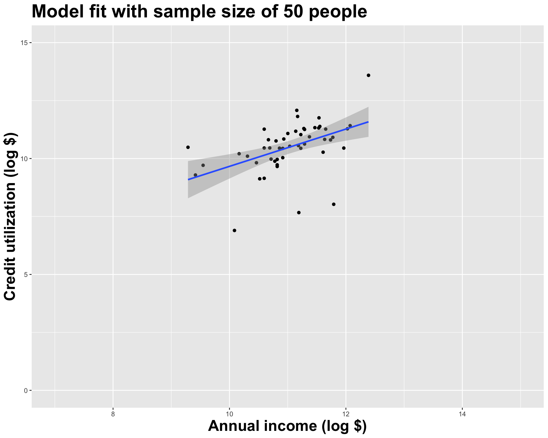

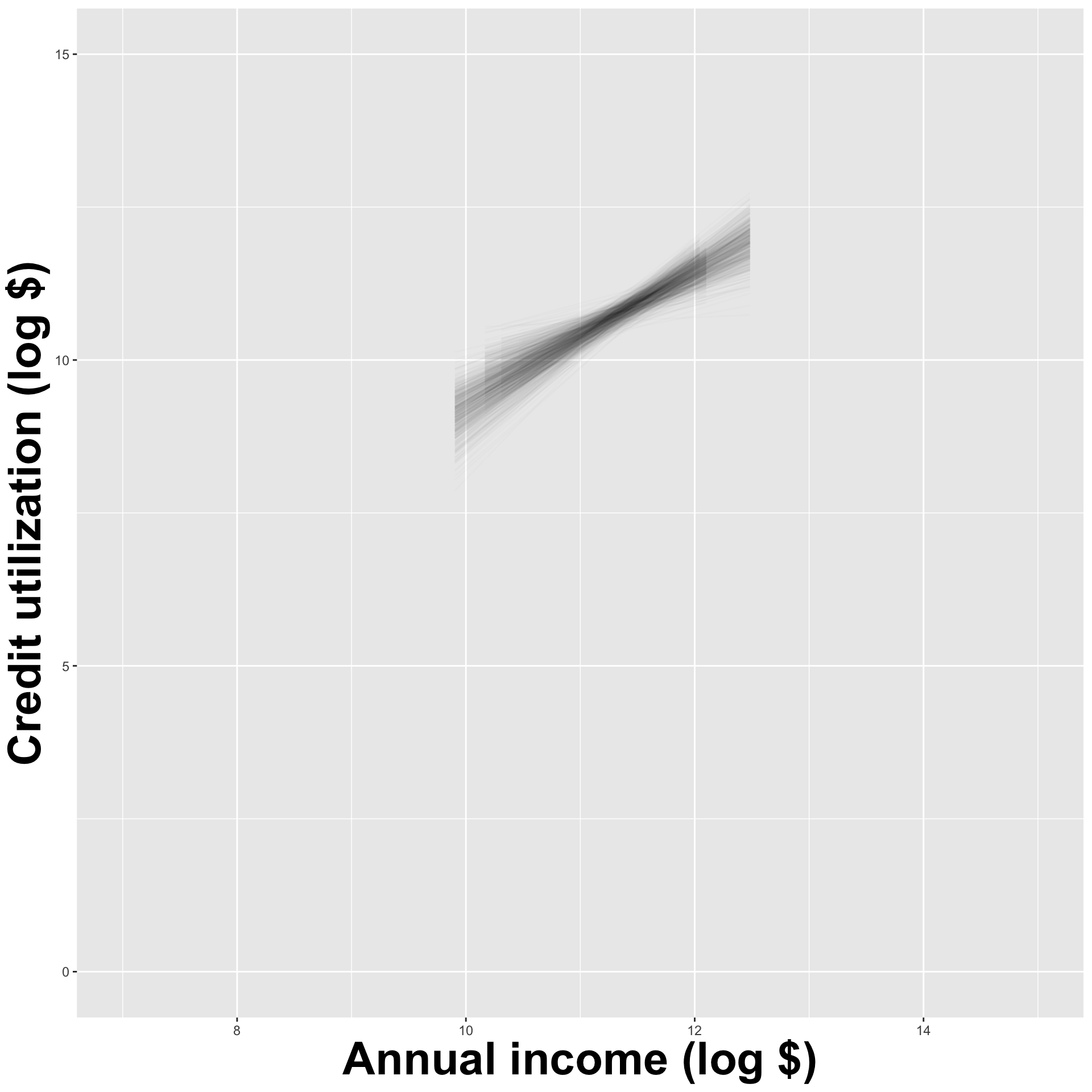
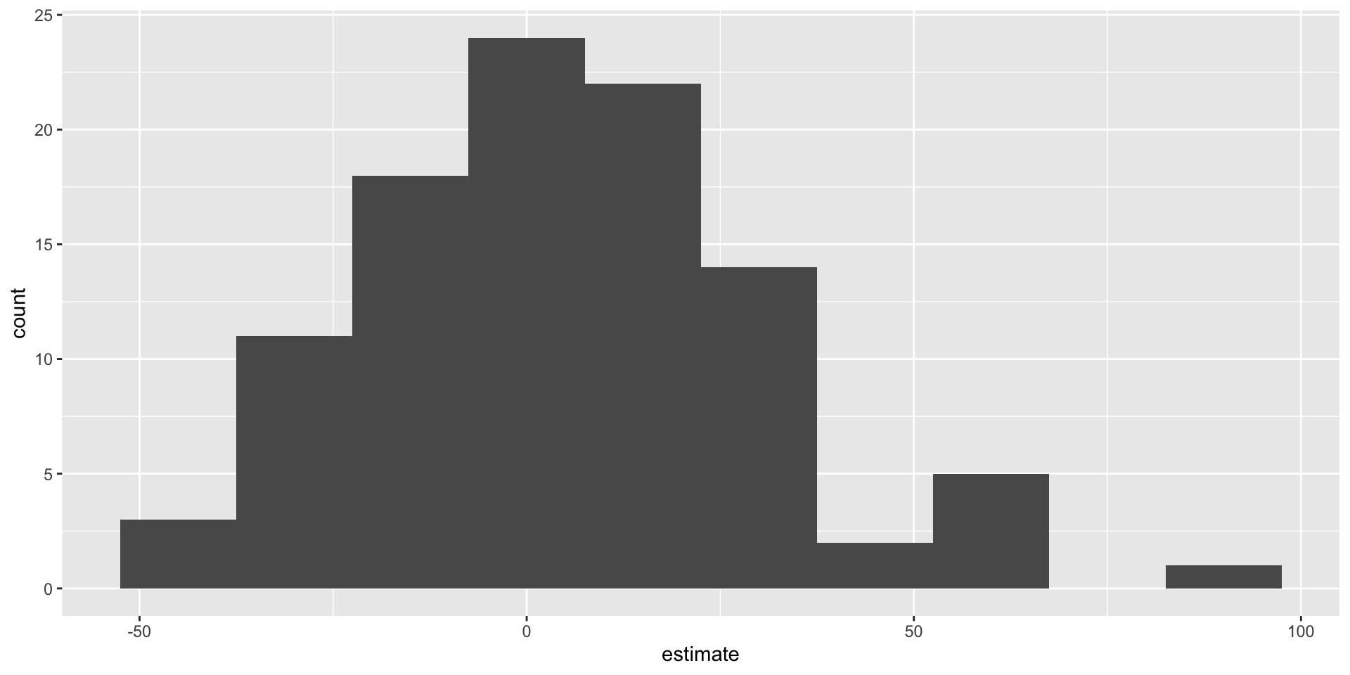
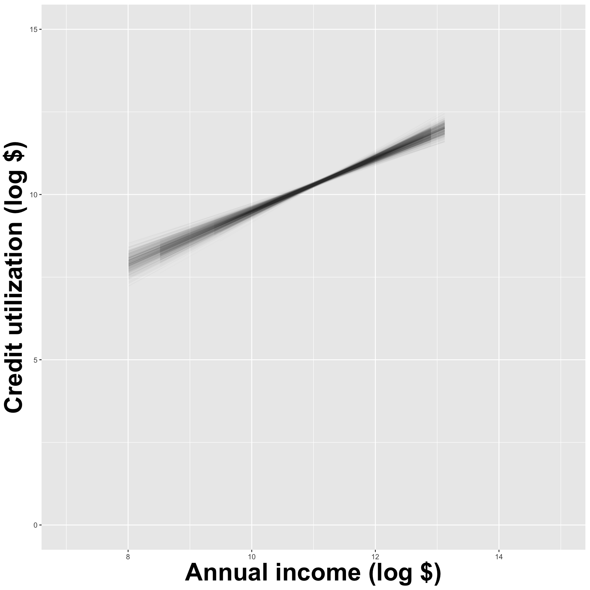
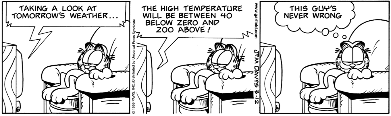
Rinse and repeat 1000 times…

Sampling uncertainty

How sensitive are the estimates to the data they are based on?

- Very? Then uncertainty is high, results are unreliable;
- Not very? Uncertainty is low, results are more reliable.

That was for n = 50. What if I was starting with n = 1000?

Sampling uncertainty decreased!

Bootstrapping

• Data collection is costly, so we have to do our best with what we already have;

• We approximate this idea of “alternative, hypothetical datasets I could have observed” by resampling our data with replacement;

• We construct a new dataset of the same size by randomly picking rows out of the original one:

  • Some rows will be duplicated;
  • Some rows will not appear at all;
  • Hence, the new dataset is different from the original;
  • Different dataset >> different estimate

• Repeat this processes hundred or thousands of times, and observe how the estimates vary as you refit the model on alternative datasets.

• This gives you a sense of the sampling variability of your estimates.

Bootstrap samples 1

Original data

# A tibble: 6 × 3
     id       x       y
  <int>   <dbl>   <dbl>
1     1  0.432   1.53  
2     2 -2.01    1.80  
3     3 -0.0467  1.43  
4     4 -1.05    0.0518
5     5  0.327   0.820 
6     6 -0.679  -0.961 

Original estimates:

# A tibble: 2 × 2
  term        estimate
  <chr>          <dbl>
1 (Intercept)   0.801 
2 x             0.0450

Sample with replacement:

# A tibble: 6 × 3
     id      x      y
  <int>  <dbl>  <dbl>
1     5  0.327  0.820
2     6 -0.679 -0.961
3     6 -0.679 -0.961
4     1  0.432  1.53 
5     6 -0.679 -0.961
6     1  0.432  1.53 

Different data >> new estimates:

# A tibble: 2 × 2
  term        estimate
  <chr>          <dbl>
1 (Intercept)    0.462
2 x              2.11 

Bootstrap samples 2

Original data

# A tibble: 6 × 3
     id       x       y
  <int>   <dbl>   <dbl>
1     1  0.432   1.53  
2     2 -2.01    1.80  
3     3 -0.0467  1.43  
4     4 -1.05    0.0518
5     5  0.327   0.820 
6     6 -0.679  -0.961 

Original estimates:

# A tibble: 2 × 2
  term        estimate
  <chr>          <dbl>
1 (Intercept)   0.801 
2 x             0.0450

Sample with replacement:

# A tibble: 6 × 3
     id       x      y
  <int>   <dbl>  <dbl>
1     2 -2.01    1.80 
2     5  0.327   0.820
3     1  0.432   1.53 
4     6 -0.679  -0.961
5     3 -0.0467  1.43 
6     2 -2.01    1.80 

Different data >> new estimates:

# A tibble: 2 × 2
  term        estimate
  <chr>          <dbl>
1 (Intercept)    0.913
2 x             -0.236

Bootstrap samples 3

Original data

# A tibble: 6 × 3
     id       x       y
  <int>   <dbl>   <dbl>
1     1  0.432   1.53  
2     2 -2.01    1.80  
3     3 -0.0467  1.43  
4     4 -1.05    0.0518
5     5  0.327   0.820 
6     6 -0.679  -0.961 

Original estimates:

# A tibble: 2 × 2
  term        estimate
  <chr>          <dbl>
1 (Intercept)   0.801 
2 x             0.0450

Sample with replacement:

# A tibble: 6 × 3
     id      x      y
  <int>  <dbl>  <dbl>
1     6 -0.679 -0.961
2     1  0.432  1.53 
3     5  0.327  0.820
4     6 -0.679 -0.961
5     6 -0.679 -0.961
6     5  0.327  0.820

Different data >> new estimates:

# A tibble: 2 × 2
  term        estimate
  <chr>          <dbl>
1 (Intercept)    0.357
2 x              1.96 

Confidence intervals

• Point estimation: report your single number best guess for the unknown quantity;

• Interval estimation: report a range, or interval, or values where you think the unknown quantity is likely to live;

  • Interval should be wide enough to capture the truth with high probability;
  • Interval should be narrow enough to be informative;

• Unfortunately, there is a trade-off. You adjust the confidence level to try to negotiate the trade-off;

• Common choices: 90%, 95%, 99%.

Precision vs. accuracy

Data: Houses in Duke Forest

• Data on houses that were sold in the Duke Forest neighborhood of Durham, NC around November 2020
• Scraped from Zillow
• Source: openintro::duke_forest

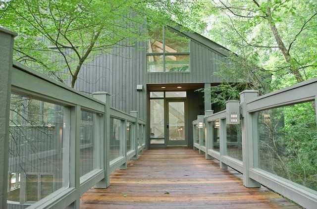
Goal: Use the area (in square feet) to understand variability in the price of houses in Duke Forest.

Modeling

df_fit <- linear_reg() |>
  fit(price ~ area, data = duke_forest)

tidy(df_fit) |>
  kable(digits = 2) # neatly format table to 2 digits

term	estimate	std.error	statistic	p.value
(Intercept)	116652.33	53302.46	2.19	0.03
area	159.48	18.17	8.78	0.00

Confidence interval for the slope

A confidence interval will allow us to make a statement like “For each additional square foot, the model predicts the sale price of Duke Forest houses to be higher, on average, by $159, plus or minus X dollars.”

Slopes of bootstrap samples

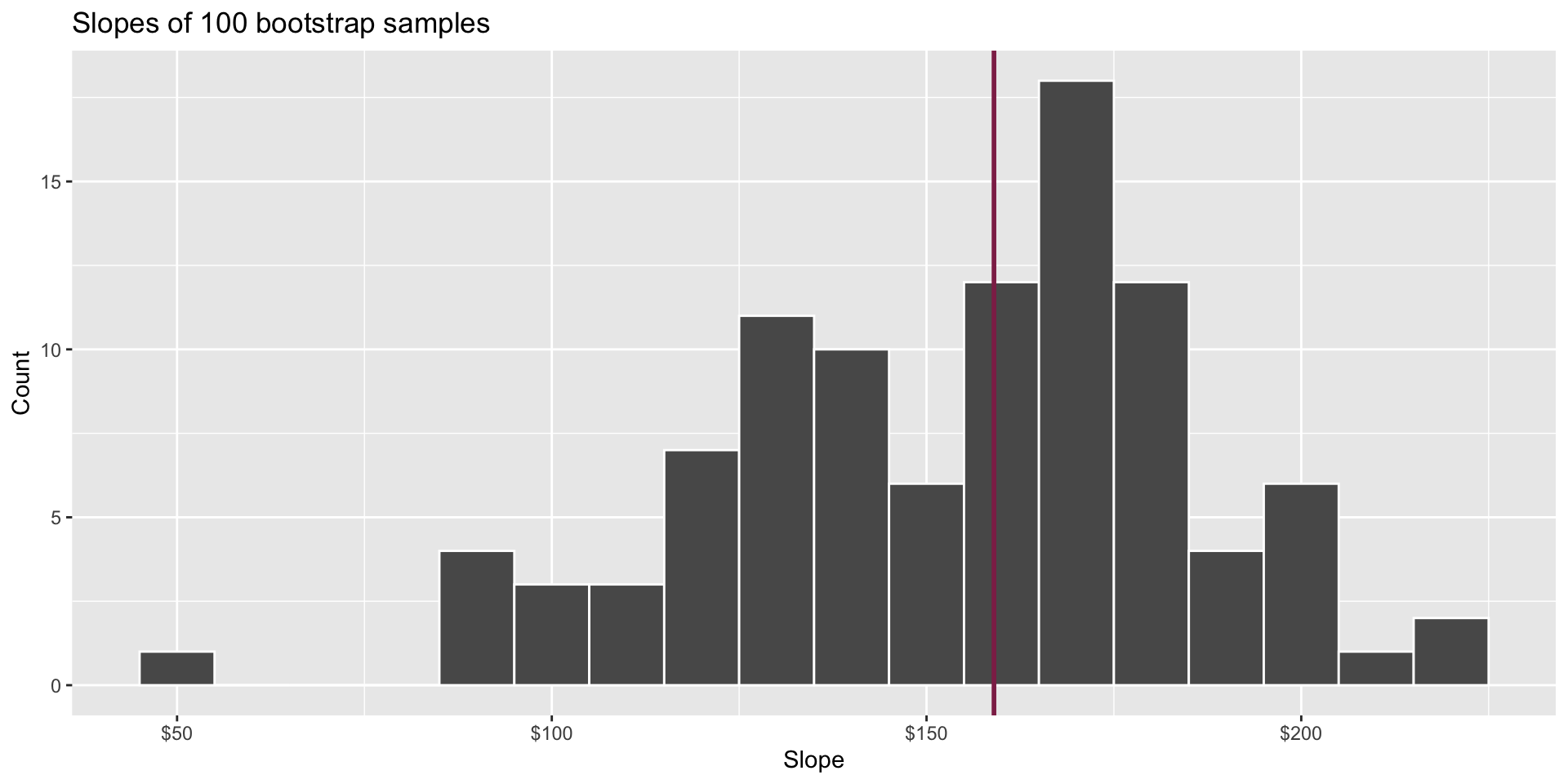
Fill in the blank: For each additional square foot, the model predicts the sale price of Duke Forest houses to be higher, on average, by $159, plus or minus ___ dollars.

Slopes of bootstrap samples

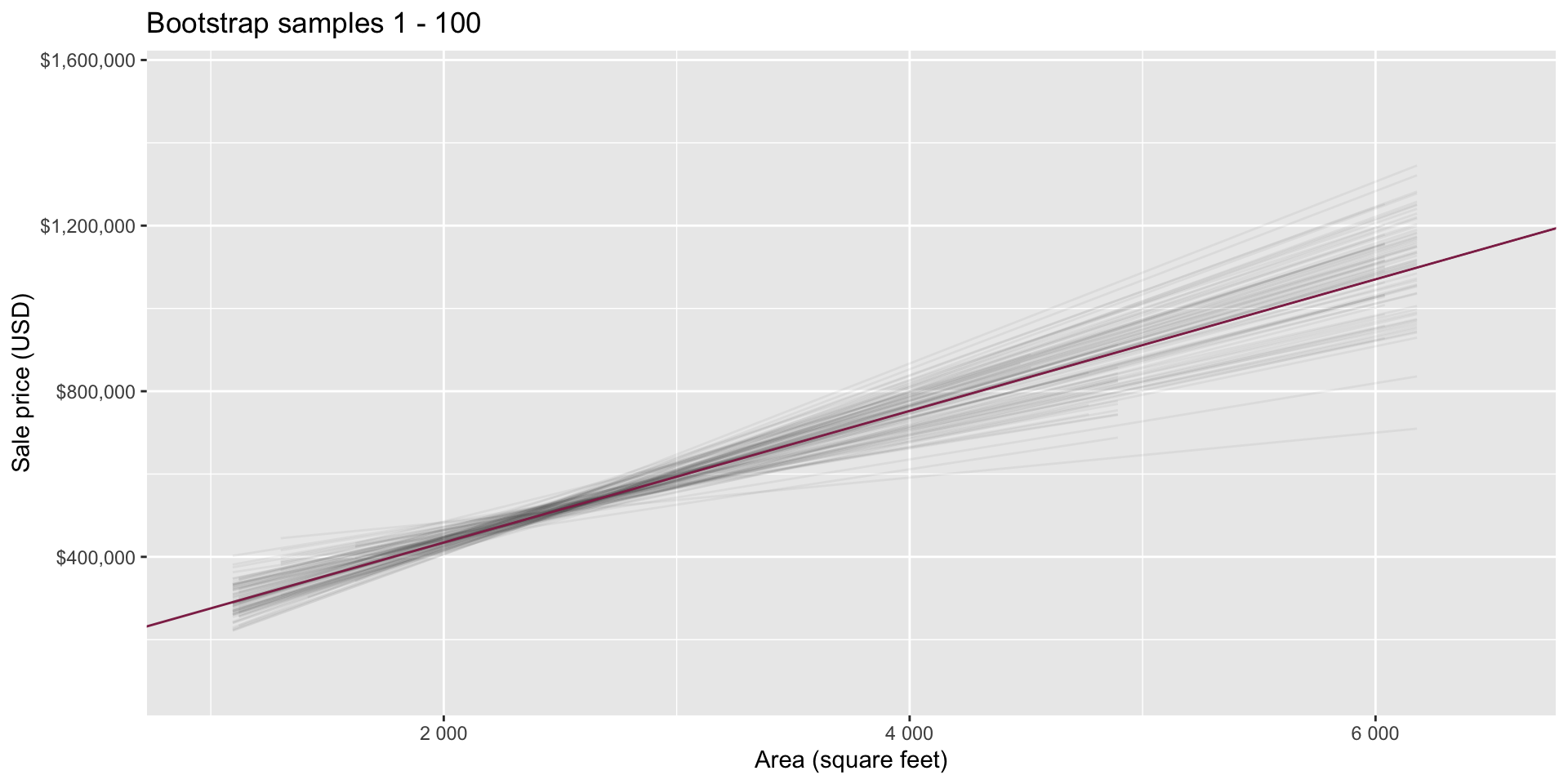
Fill in the blank: For each additional square foot, we expect the sale price of Duke Forest houses to be higher, on average, by $159, plus or minus ___ dollars.

Confidence level

How confident are you that the true slope is between $0 and $250? How about $150 and $170? How about $90 and $210?

95% confidence interval

• A 95% confidence interval is bounded by the middle 95% of the bootstrap distribution
• We are 95% confident that for each additional square foot, the model predicts the sale price of Duke Forest houses to be higher, on average, by $90.43 to $205.77.

Where do the bounds come from?

• Think IQR! 50% of the bootstrap distribution is between the 25% quantile on the left and the 75% quantile on the right. But we want more than 50%

• 90% of the bootstrap distribution is between the 5% quantile on the left and the 95% quantile on the right;

• 95% of the bootstrap distribution is between the 2.5% quantile on the left and the 97.5% quantile on the right;

• And so on.

Computing the CI for the slope I

Calculate the observed slope:

observed_fit <- duke_forest |>
  specify(price ~ area) |>
  fit()

observed_fit

# A tibble: 2 × 2
  term      estimate
  <chr>        <dbl>
1 intercept  116652.
2 area          159.

Computing the CI for the slope II

Take 100 bootstrap samples and fit models to each one:

set.seed(1120)

boot_fits <- duke_forest |>
  specify(price ~ area) |>
  generate(reps = 100, type = "bootstrap") |>
  fit()

boot_fits

# A tibble: 200 × 3
# Groups:   replicate [100]
   replicate term      estimate
       <int> <chr>        <dbl>
 1         1 intercept   47819.
 2         1 area          191.
 3         2 intercept  144645.
 4         2 area          134.
 5         3 intercept  114008.
 6         3 area          161.
 7         4 intercept  100639.
 8         4 area          166.
 9         5 intercept  215264.
10         5 area          125.
# ℹ 190 more rows

Computing the CI for the slope III

Percentile method: Compute the 95% CI as the middle 95% of the bootstrap distribution:

get_confidence_interval(
  boot_fits, 
  point_estimate = observed_fit, 
  level = 0.95,
  type = "percentile" # default method
)

# A tibble: 2 × 3
  term      lower_ci upper_ci
  <chr>        <dbl>    <dbl>
1 area          92.1     223.
2 intercept -36765.   296528.

Computing the CI for the slope IV

If we did it manually…

boot_fits |>
  filter(term == "area") |>
  ungroup() |>
  summarize(
    lower_ci = quantile(estimate, 0.025),
    upper_ci = quantile(estimate, 0.975),
  )

# A tibble: 1 × 2
  lower_ci upper_ci
     <dbl>    <dbl>
1     92.1     223.

Changing confidence level

How would you modify the following code to calculate a 90% confidence interval? How would you modify it for a 99% confidence interval?

get_confidence_interval(
  boot_fits, 
  point_estimate = observed_fit, 
  level = 0.95,
  type = "percentile"
)

# A tibble: 2 × 3
  term      lower_ci upper_ci
  <chr>        <dbl>    <dbl>
1 area          92.1     223.
2 intercept -36765.   296528.

Changing confidence level

## confidence level: 90%
get_confidence_interval(
  boot_fits, point_estimate = observed_fit, 
  level = 0.90, type = "percentile"
)

# A tibble: 2 × 3
  term      lower_ci upper_ci
  <chr>        <dbl>    <dbl>
1 area          104.     212.
2 intercept  -24380.  256730.

## confidence level: 99%
get_confidence_interval(
  boot_fits, point_estimate = observed_fit, 
  level = 0.99, type = "percentile"
)

# A tibble: 2 × 3
  term      lower_ci upper_ci
  <chr>        <dbl>    <dbl>
1 area          56.3     226.
2 intercept -61950.   370395.

Recap

• Population: Complete set of observations of whatever we are studying, e.g., people, tweets, photographs, etc. (population size = \(N\))

• Sample: Subset of the population, ideally random and representative (sample size = \(n\))

• Sample statistic \(\ne\) population parameter, but if the sample is good, it can be a good estimate

• Statistical inference: Discipline that concerns itself with the development of procedures, methods, and theorems that allow us to extract meaning and information from data that has been generated by stochastic (random) process

• We report the estimate with a confidence interval, and the width of this interval depends on the variability of sample statistics from different samples from the population

• Since we can’t continue sampling from the population, we bootstrap from the one sample we have to estimate sampling variability

Hypothesis testing

Hypothesis testing

A hypothesis test is a statistical technique used to evaluate competing claims using data

• Null hypothesis, \(H_0\): An assumption about the population. “There is nothing going on.”

• Alternative hypothesis, \(H_A\): A research question about the population. “There is something going on”.

Note: Hypotheses are always at the population level!

Setting hypotheses

• Null hypothesis, \(H_0\): “There is nothing going on.” The slope of the model for predicting the prices of houses in Duke Forest from their areas is 0, \(\beta_1 = 0\).

• Alternative hypothesis, \(H_A\): “There is something going on”. The slope of the model for predicting the prices of houses in Duke Forest from their areas is different than, \(\beta_1 \ne 0\).

Hypothesis testing “mindset”

• Assume you live in a world where null hypothesis is true: \(\beta_1 = 0\).

• Ask yourself how likely you are to observe the sample statistic, or something even more extreme, in this world: \(P(b_1 \leq 159.48~or~b_1 \geq 159.48 | \beta_1 = 0)\) = ?

Hypothesis testing as a court trial

• Null hypothesis, \(H_0\): Defendant is innocent

• Alternative hypothesis, \(H_A\): Defendant is guilty

• Present the evidence: Collect data

• Judge the evidence: “Could these data plausibly have happened by chance if the null hypothesis were true?”
  • Yes: Fail to reject \(H_0\)
  • No: Reject \(H_0\)

Hypothesis testing as medical diagnosis

• Null hypothesis, \(H_0\): patient is fine

• Alternative hypothesis, \(H_A\): patient is sick

• Present the evidence: Collect data

• Judge the evidence: “Could these data plausibly have happened by chance if the null hypothesis were true?”
  • Yes: Fail to reject \(H_0\)
  • No: Reject \(H_0\)

Hypothesis testing framework

• Start with a null hypothesis, \(H_0\), that represents the status quo

• Set an alternative hypothesis, \(H_A\), that represents the research question, i.e. what we’re testing for

• Conduct a hypothesis test under the assumption that the null hypothesis is true and calculate a p-value (probability of observed or more extreme outcome given that the null hypothesis is true)

  • if the test results suggest that the data do not provide convincing evidence for the alternative hypothesis, stick with the null hypothesis
  • if they do, then reject the null hypothesis in favor of the alternative

Calculate observed slope

… which we have already done:

observed_fit <- duke_forest |>
  specify(price ~ area) |>
  fit()

observed_fit

# A tibble: 2 × 2
  term      estimate
  <chr>        <dbl>
1 intercept  116652.
2 area          159.

Simulate null distribution

set.seed(20241118)
null_dist <- duke_forest |>
  specify(price ~ area) |>
  hypothesize(null = "independence") |>
  generate(reps = 100, type = "permute") |>
  fit()

View null distribution

null_dist

# A tibble: 200 × 3
# Groups:   replicate [100]
   replicate term        estimate
       <int> <chr>          <dbl>
 1         1 intercept 547294.   
 2         1 area           4.54 
 3         2 intercept 568599.   
 4         2 area          -3.13 
 5         3 intercept 561547.   
 6         3 area          -0.593
 7         4 intercept 526286.   
 8         4 area          12.1  
 9         5 intercept 651476.   
10         5 area         -33.0  
# ℹ 190 more rows

Visualize null distribution

null_dist |>
  filter(term == "area") |>
  ggplot(aes(x = estimate)) +
  geom_histogram(binwidth = 15)

Visualize null distribution (alternative)

visualize(null_dist) +
  shade_p_value(obs_stat = observed_fit, direction = "two-sided")

Get p-value

null_dist |>
  get_p_value(obs_stat = observed_fit, direction = "two-sided")

# A tibble: 2 × 2
  term      p_value
  <chr>       <dbl>
1 area            0
2 intercept       0

Make a decision

Based on the p-value calculated, what is the conclusion of the hypothesis test?

Sometimes the test will be wrong

Think about the judge

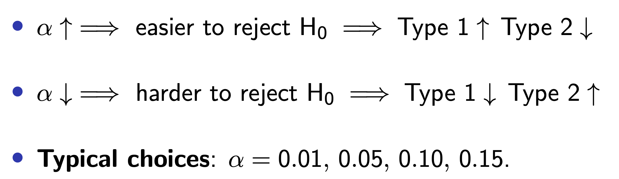
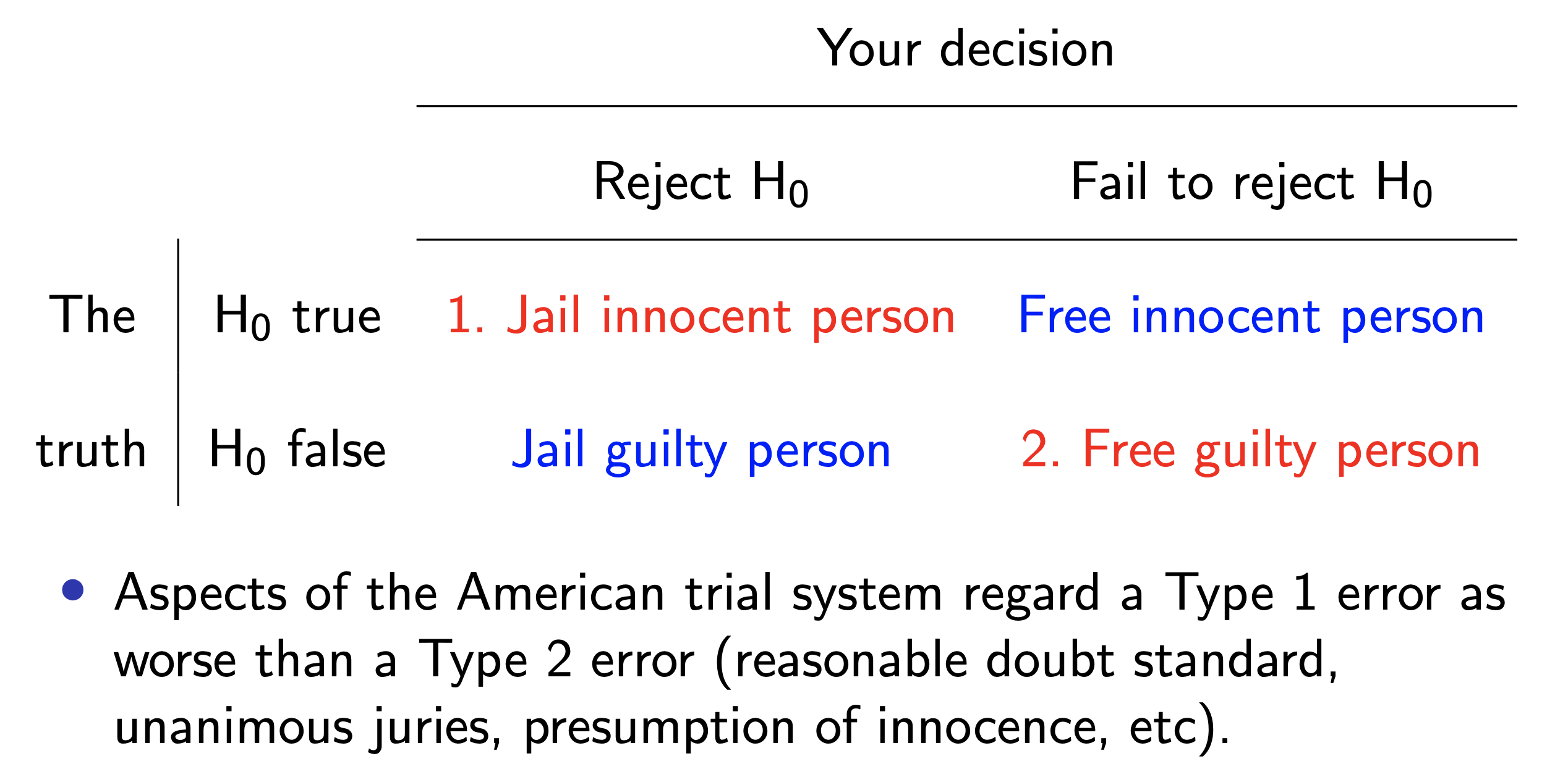
\(H_0\) person innocent vs \(H_A\) person guilty

Think about the doctor

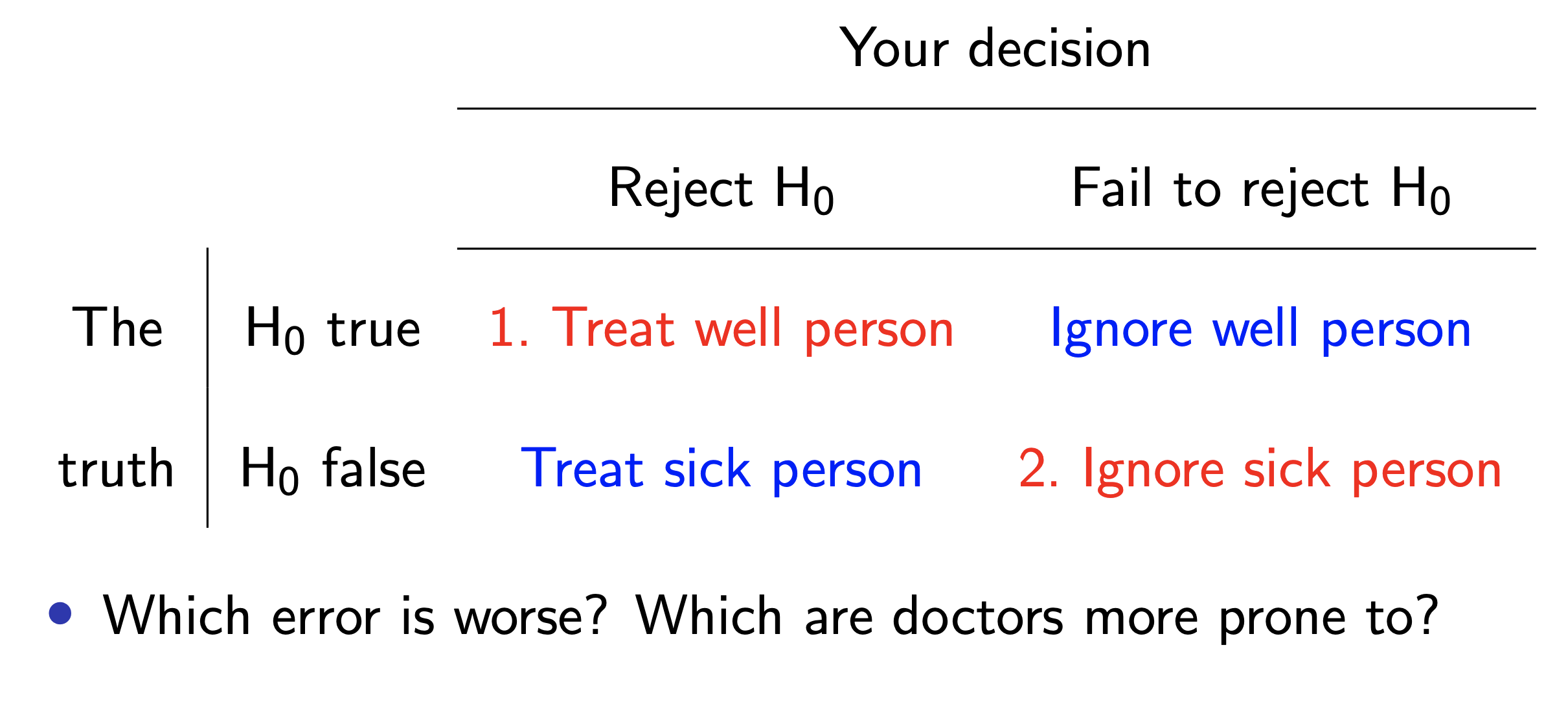
\(H_0\) person well vs \(H_A\) person sick.

How do we negotiate the trade-off?

Pick a threshold \(\alpha\in[0,\,1]\) called the discernibility level and threshold the \(p\)-value:

• If \(p\text{-value} < \alpha\), reject null and accept alternative;
• If \(p\text{-value} \geq \alpha\), fail to reject null;