Lab 4

John Zito

Duke University
STA 199 Spring 2025

2025-02-10

While you wait… get your repo ready

• Log in to RStudio (via your container)

  • Go to https://cmgr.oit.duke.edu/containers and click STA198-199

• Clone the repo & start a new RStudio project

  • Go to the course organization at github.com/sta199-s25 organization on GitHub. Click on the repo with the prefix lab-4.

  • Click on the green CODE button and select Use SSH. Click on the clipboard icon to copy the repo URL.

  • In RStudio, go to File ➛ New Project ➛Version Control ➛ Git to clone your Lab 4 repo.

• Update the YAML

  • In lab-4.qmd, update the author field to your name, Render your document, and examine the changes. Then, in the Git pane, click on Diff to view your changes, add a commit message (e.g., “Added author name”), and click Commit. Then, Push the changes to your GitHub repository and, in your browser, confirm that these changes have indeed propagated to your repository.

Should look at Marie’s notes again (from email on 1/22/25). There are more notes there to incorporate, especially in earlier labs with the motivation.

A review

You have learned a lot thus far

• Git/GitHub

• R

  • Plot related functions

    ggplot(), aes(), geom_boxplot(), geom_point(), geom_histogram(), geom_smooth(), geom_line(), geom_beeswarm(), labs(), theme_minimal(), theme() scale_x_continuous(), scale_color_manual()

  • More functions

    glimpse(), nrow(), ncol(), dim(), slice_head(), filter(), arrange(), relocate(), if_else(), case_when(), count(), group_by(), ungroup(), read_csv(), separate(), mutate(), summarize(), pivot_*(), *_join()

Git/Github: had lots of practice pulling, committing and pushing changes to update your repos on GitHub.

R: These functions were taken from ae-02 to ae-06 and the prepare videos (a good places to practice and refresh what you’ve learned).

(optional, may not be enough time – can transition by stating let’s talk about a few of these in more detail) Have students raise hands to ask state these functions do (with an emphasis on those under more functions) – just for 5 or so functions. Hopefully, multiple students raise their hands. Otherwise you can simply move on.

Transition: now let’s do a more thorough review of some of these functions

mutate() and summarize()

 

 

• mutate(): modifies existing data frame – creates new columns (i.e., variables) or modifies existing columns. Note that the number of rows does not change.

 

• summarize(): creates a new data frame – returns one for for each combination of grouping variables. If there is no grouping it will have a single row summarizing all observations

Example: Set up

library(tidyverse)
library(knitr)

df <- tibble(
  col_1 = c("A", "A", "A", "B", "B"),
  col_2 = c("X", "Y", "X", "X", "Y"),
  col_3 = c(1, 2, 3, 4, 5)
)

df #this is used to display the data frame

# A tibble: 5 × 3
  col_1 col_2 col_3
  <chr> <chr> <dbl>
1 A     X         1
2 A     Y         2
3 A     X         3
4 B     X         4
5 B     Y         5

What would be the result of the following code? # rows? # cols? column/variable names?

df |>
  mutate(med_col_3 = median(col_3))


df |>
  summarize(med_col_3 = median(col_3))

HAVE THE STUDENTS GUESS how many rows, columns, what the variable names will be?

mutate: number of rows does not change, number of columns increases by 1 (med_col_3). Could have also introduced more new variables within the mutate function using commas,

df |>
  mutate(
    med_col_3 = median(col_3),
    mean_col_3 = mean(col_3)
    )

summarize: there is only 1 row and 1 col! (this is a much different data frame than df!). Could have had more columns/variables if added more variables within summarize function using commas. [same as above, just replace mutate with summarize]

assignment: have the students guess

Example: no groups

mutate()

df |>
  mutate(med_col_3 = median(col_3))

# A tibble: 5 × 4
  col_1 col_2 col_3 med_col_3
  <chr> <chr> <dbl>     <dbl>
1 A     X         1         3
2 A     Y         2         3
3 A     X         3         3
4 B     X         4         3
5 B     Y         5         3

summarize()

df |>
  summarize(med_col_3 = median(col_3))

# A tibble: 1 × 1
  med_col_3
      <dbl>
1         3

We did not assign any new or existing data frames (e.g., no ??? <-). In particular, we did not write over df (i.e., no df <-), so what will be the result of the following code?

df

mutate: there was no column named med_col_3, so a new column was created

summarize: there is no grouping, so there is one output summarizing so the median is computed over all of the original rows of the data (five rows in this example)

assignment: have the students guess

Example: assignment

• It’s the same as when it was originally assigned. It has not been overwritten!

df 

# A tibble: 5 × 3
  col_1 col_2 col_3
  <chr> <chr> <dbl>
1 A     X         1
2 A     Y         2
3 A     X         3
4 B     X         4
5 B     Y         5

• We will often write a single pipeline and show the result, i.e., no assignment.

• If you will need to refer to the data frame later, it might be a good idea to assign a name to the data frame. Otherwise, see the result and continue on.

  Note: if you assign the new/updated data frame, the result does not appear in the Console or the rendered document! (Type the name of the variable, e.g., df as shown above, to display the data frame.)

Example: with groups

What if there is grouping?

# group by 1 variable
df |>
  group_by(col_1) |>
  mutate(med_col_3 = median(col_3))


df |>
  group_by(col_1) |>
  summarize(med_col_3 = median(col_3))

# group by 2 variables
df |>
  group_by(col_1, col_2) |>
  mutate(med_col_3 = median(col_3))


df |>
  group_by(col_1, col_2) |>
  summarize(med_col_3 = median(col_3))

If you aren’t sure, try it out and see what happens (e.g., use data frame from Lab 3, Part 1).

I would have written this out in Lab 3 prep. But there is other stuff to get to for Lab 4 prep that I didn’t want this to take up too much of the time. Plus, by now they saw what happened already in Lab 3.

Also, make a comment about the grouping when expanding upon this next semester.

pivot_*()

• Pivoting reshapes the data frame.

• pivot_longer makes the updated data frame longer (i.e., fewer columns)

• pivot_wider makes the updated data frame wider (i.e., more columns)

Example: pivot_*()

Let’s examine the number of hours people slept during the week.

How do we go from this…

ppl	Mon	Tues	Weds	Thurs	Fri
person1	8	7	6	10	8
person2	7	5	4	6	7

…to this?

ppl	day	hours
person1	Mon	8
person1	Tues	7
person1	Weds	6
person1	Thurs	10
person1	Fri	8
person2	Mon	7
person2	Tues	5
person2	Weds	4
person2	Thurs	6
person2	Fri	7

df_longer <- df |>
  pivot_longer(
    cols = -ppl,
    names_to = "day",
    values_to = "hours"
  )

pivot_longer() or pivot_wider()? Have the students vote. pivot_longer()!

What should the arguments be? (Go through the argument discussion first, then reveal the result toward the end – giving them enough time to look at it for visual learners)

cols = -ppl: cols – the columns to be pivoted (i.e., stacked into rows). in this case all of the columns except ppl (ppl column/variable remains)

names_to = "day": names_to – the new column/variable name for the original column/variable names [point to the Mon, Tues, Weds, … in the original table]

values_to = "hours": names_to – the new column/variable name for the values from the original data [point to the hours of sleep in the original table]

Note that the column/variable names “day” and “hours” did not exist until using pivot_longer()

Question: What if I hadn’t assigned the result to df_longer? What would the display look like and what would the df data frame be if I had deleted the df_longer <- portion of the code?

Answer: The console would show the data frame df_longer (though it wouldn’t be named – it would just read # A tibble: 10 x 3 and so on), and df remains unchanged. It’s the same wide (2 x 6) tibble it originally was defined as.

*_join()

• Typically we use *_join() to merge data from two data frames (e.g., left_join(), right_join(), full_join(), inner_join()), i.e., create a new data frames with more columns/variables.

  For example, there is useful info in two data frames: x and y. We want to create a new data frame which includes variables from both (e.g., data frame x has student ID numbers and student names and data frame y has student ID numbers and email addresses).

• Sometimes we use *_join() to filter rows/observations, e.g., find the rows from one data frame that do (or do not) exist in another data frame (e.g., semi_join(), anti_join())

• Let’s focus on the joins that merge data…

Example: *_join() setup

For the next few slides…

x <- tibble(
  id = c(1, 2, 3),
  value_x = c("x1", "x2", "x3")
  )

x

# A tibble: 3 × 2
     id value_x
  <dbl> <chr>  
1     1 x1     
2     2 x2     
3     3 x3     

y <- tibble(
  id = c(1, 2, 4),
  value_y = c("y1", "y2", "y4")
  )

y

# A tibble: 3 × 2
     id value_y
  <dbl> <chr>  
1     1 y1     
2     2 y2     
3     4 y4     

left_join()

left_join(x, y)

# A tibble: 3 × 3
     id value_x value_y
  <dbl> <chr>   <chr>  
1     1 x1      y1     
2     2 x2      y2     
3     3 x3      <NA>   

Keep all rows from left data frame.

right_join()

right_join(x, y)

# A tibble: 3 × 3
     id value_x value_y
  <dbl> <chr>   <chr>  
1     1 x1      y1     
2     2 x2      y2     
3     4 <NA>    y4     

  Keep all rows from right data frame.

full_join()

full_join(x, y)

# A tibble: 4 × 3
     id value_x value_y
  <dbl> <chr>   <chr>  
1     1 x1      y1     
2     2 x2      y2     
3     3 x3      <NA>   
4     4 <NA>    y4     

 

Keep all rows from both data frames.

inner_join()

inner_join(x, y)

# A tibble: 2 × 3
     id value_x value_y
  <dbl> <chr>   <chr>  
1     1 x1      y1     
2     2 x2      y2     

 

Keep all rows that exist in both data frames.

Example: *_join() more info

• We could also use *_join() within a pipeline.

x |>
  left_join(y)

• Which data frame is on the left and which is on the right? x or y?

• The above code is equivalent to left_join(x, y) since the result before the pipe |> is passed as the first argument to the function after the pipe.

• In this example x has 2 variables: id and value_x and y has 2 variables: id and value_x, so there was only one common variable between x and y – id. We could have been more explicit and used the following code

left_join(x, y, by = join_by(id))

# or alternatively

left_join(x, y, by = join_by(id == id))

The first option is useful when there are multiple matching columns [and by default *_join() will use all variables in common across x and y] but perhaps only one of interest (e.g., student_ids and email_address – the same student could have multiple email addresses but you want each student to be one row/observation, so you would use by = join_by(student_ids)).

The second option is used when the variables do not share the same variable name but are referring to the same information, e.g., id == student_id.

Backup info: why piping? piping is much easier to read (can see all data frame manipulation at once – and it isn’t an extreme run-on sentence, e.g., summarize(mutatate(), arg, arg, arg….); also, potentially less having to save and remember intermediate variables) – both for you and others.

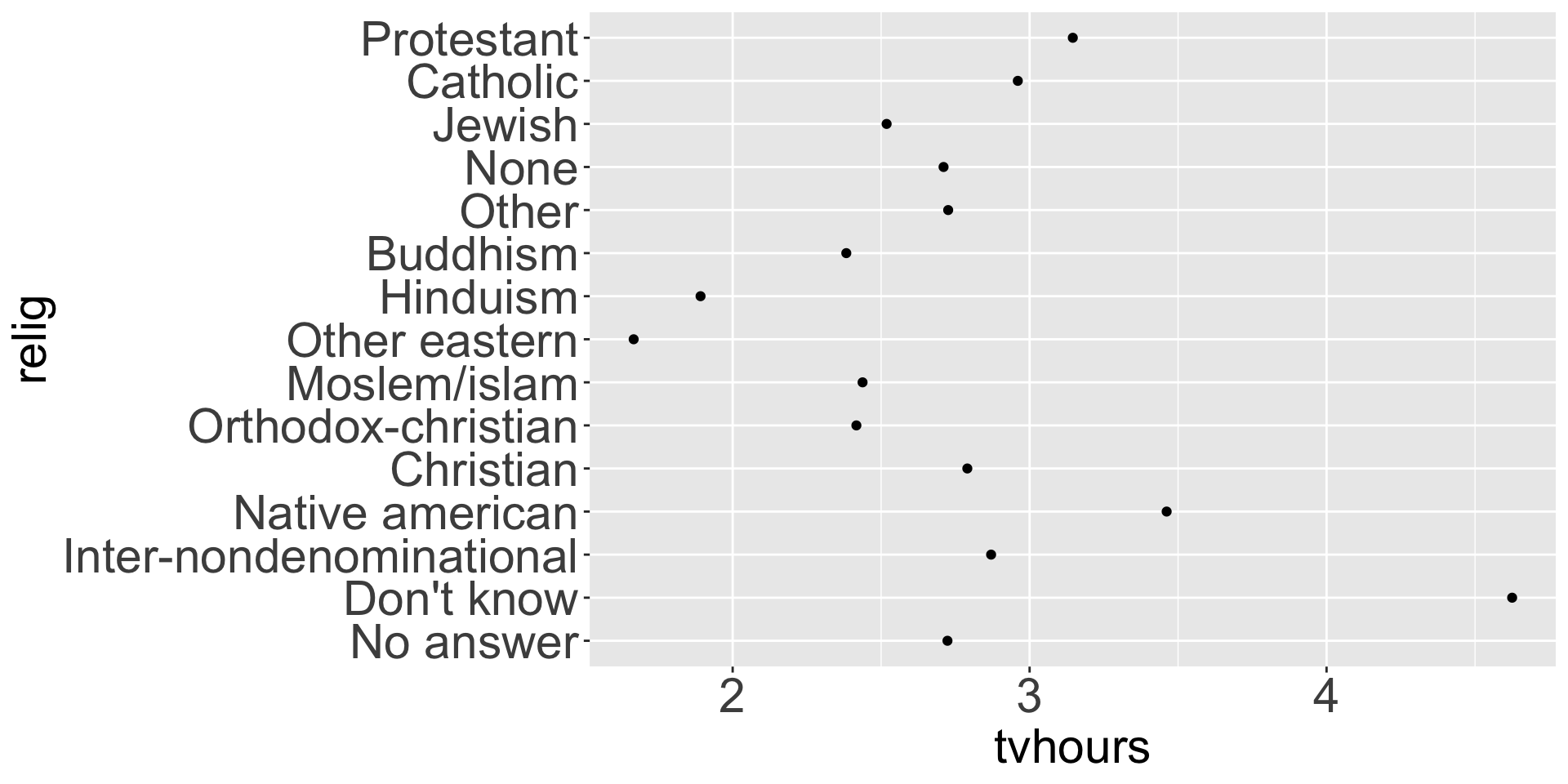
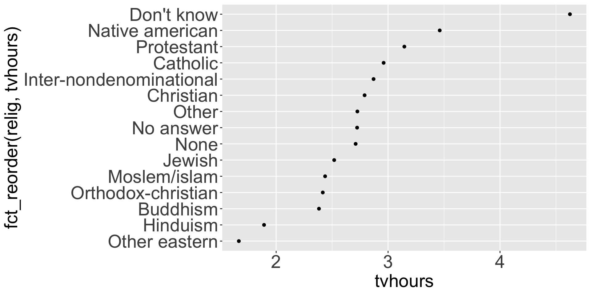
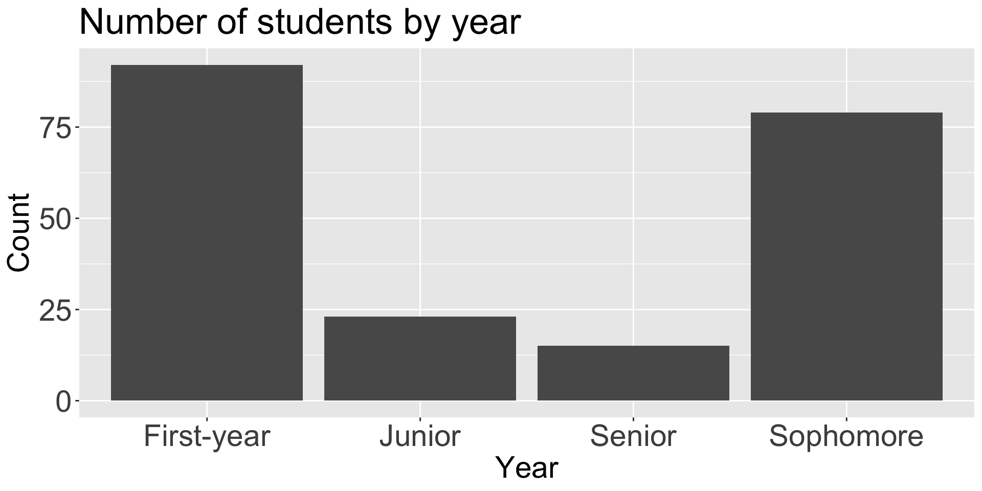
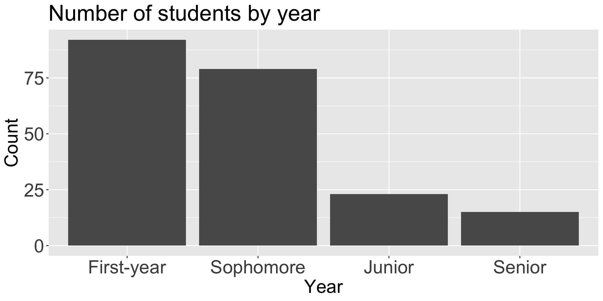
Factors

• Factors are used for categorical variables, e.g., days of the week; religion; low, mid, high

• Very helpful for ordering (i.e., when numerical and alphabetical ordering don’t cut it!)

• Examples

  • Friday, Monday, Saturday, Sunday, Tuesday, Thursday, Wednesday

  • Apr, Feb, Jan, July, Jun, Mar, May

  • Agree, Disagree, Neither agree nor disagree, Strongly agree, Strongly disagree

  • Example below (from prepare [r4ds] chp 16.4)

Factor example

Recall from Thursday’s lecture

survey |>
  mutate(
    year = fct_relevel(year, "First-year", "Sophomore", "Junior", "Senior")
    ) |>
  ggplot(aes(x = year)) +
  geom_bar() + 
  labs(
    title = "Number of students by year",
    x = "Year",
    y = "Count"
  )

How is the x-axis ordered in the left and right plots?

Recall from Thursday’s lecture, using context we know about the data it’s more appropriate for the year to have the order: first-year, sophomore, junior, senior and we used fct_revel to manually (we explicityly wrote out the order) change the ordering of the year variable.

The data is ordered alphabetically on the left (default for ggplot to order numerically or alphabetically).

Ordered according to fct_relevel ordering on the right

Also that fct_revel did two things: it made the year variable a factor AND it set the order. (aside if asked) Note that ggplot will by default coerce the character variable to be a factor. Regardless if you assigned the data frame after running fct_revel it will be a factor (and you don’t need to separately use the factor() function).

This week’s lab

• Gain more experience with joining and pivoting data frames; and modifying the order of factors.

• Review Quarto cell options

• Learn to read data in from Excel spreadsheets (will learn more on Tuesday about this)

• Datasets

  • More inflation!

  • 2020 and 2024 US Olympic Team rosters

  • Survey regarding medical marijuana in NC

  • mtcars from 1974 Motor Trend US magazine