Midterm 2 Practice Questions

Solutions

See here.

Part 1 - Blizzard

In 2020, employees of Blizzard Entertainment circulated a spreadsheet to anonymously share salaries and recent pay increases amidst rising tension in the video game industry over wage disparities and executive compensation. (Source: Blizzard Workers Share Salaries in Revolt Over Pay)

The name of the data frame used for this analysis is blizzard_salary and the variables are:

• percent_incr: Raise given in July 2020, as percent increase with values ranging from 1 (1% increase to 21.5 (21.5% increase)

• salary_type: Type of salary, with levels Hourly and Salaried

• annual_salary: Annual salary, in USD, with values ranging from $50,939 to $216,856.

• performance_rating: Most recent review performance rating, with levels Poor, Successful, High, and Top. The Poor level is the lowest rating and the Top level is the highest rating.

The top ten rows of blizzard_salary are shown below:

# A tibble: 409 × 4
   percent_incr salary_type annual_salary performance_rating
          <dbl> <chr>               <dbl> <chr>             
 1          1   Salaried               1  High              
 2          1   Salaried               1  Successful        
 3          1   Salaried               1  High              
 4          1   Hourly             33987. Successful        
 5         NA   Hourly             34798. High              
 6         NA   Hourly             35360  <NA>              
 7         NA   Hourly             37440  <NA>              
 8          0   Hourly             37814. <NA>              
 9          4   Hourly             41101. Top               
10          1.2 Hourly             42328  <NA>              
# ℹ 399 more rows

Question 1

You fit a model for predicting raises (percent_incr) from salaries (annual_salary). We’ll call this model raise_1_fit. A tidy output of the model is shown below.

# A tibble: 2 × 5
  term           estimate  std.error statistic   p.value
  <chr>             <dbl>      <dbl>     <dbl>     <dbl>
1 (Intercept)   1.87      0.432           4.33 0.0000194
2 annual_salary 0.0000155 0.00000452      3.43 0.000669 

Which of the following is the best interpretation of the slope coefficient?

1. For every additional $1,000 of annual salary, the model predicts the raise to be higher, on average, by 1.55%.
2. For every additional $1,000 of annual salary, the raise goes up by 0.0155%.
3. For every additional $1,000 of annual salary, the model predicts the raise to be higher, on average, by 0.0155%.
4. For every additional $1,000 of annual salary, the model predicts the raise to be higher, on average, by 1.87%.

Question 2

You then fit a model for predicting raises (percent_incr) from salaries (annual_salary) and performance ratings (performance_rating). We’ll call this model raise_2_fit. Which of the following is definitely true based on the information you have so far?

1. Intercept of raise_2_fit is higher than intercept of raise_1_fit.
2. Slope of raise_2_fit is higher than RMSE of raise_1_fit.
3. Adjusted \(R^2\) of raise_2_fit is higher than adjusted \(R^2\) of raise_1_fit.
4. \(R^2\) of raise_2_fit is higher \(R^2\) of raise_1_fit.

Question 3

The tidy model output for the raise_2_fit model you fit is shown below.

# A tibble: 5 × 5
  term                            estimate  std.error statistic  p.value
  <chr>                              <dbl>      <dbl>     <dbl>    <dbl>
1 (Intercept)                   3.55       0.508           6.99 1.99e-11
2 annual_salary                 0.00000989 0.00000436      2.27 2.42e- 2
3 performance_ratingPoor       -4.06       1.42           -2.86 4.58e- 3
4 performance_ratingSuccessful -2.40       0.397          -6.05 4.68e- 9
5 performance_ratingTop         2.99       0.715           4.18 3.92e- 5

When your teammate sees this model output, they remark “The coefficient for performance_ratingSuccessful is negative, that’s weird. I guess it means that people who get successful performance ratings get lower raises.” How would you respond to your teammate?

Question 4

Ultimately, your teammate decides they don’t like the negative slope coefficients in the model output you created (not that there’s anything wrong with negative slope coefficients!), does something else, and comes up with the following model output.

# A tibble: 5 × 5
  term                            estimate  std.error statistic    p.value
  <chr>                              <dbl>      <dbl>     <dbl>      <dbl>
1 (Intercept)                  -0.511      1.47          -0.347 0.729     
2 annual_salary                 0.00000989 0.00000436     2.27  0.0242    
3 performance_ratingSuccessful  1.66       1.42           1.17  0.242     
4 performance_ratingHigh        4.06       1.42           2.86  0.00458   
5 performance_ratingTop         7.05       1.53           4.60  0.00000644

Unfortunately they didn’t write their code in a Quarto document, instead just wrote some code in the Console and then lost track of their work. They remember using the fct_relevel() function and doing something like the following:

blizzard_salary <- blizzard_salary |>
  mutate(performance_rating = fct_relevel(performance_rating, ___))

What should they put in the blanks to get the same model output as above?

1. “Poor”, “Successful”, “High”, “Top”
2. “Successful”, “High”, “Top”
3. “Top”, “High”, “Successful”, “Poor”
4. Poor, Successful, High, Top

Question 5

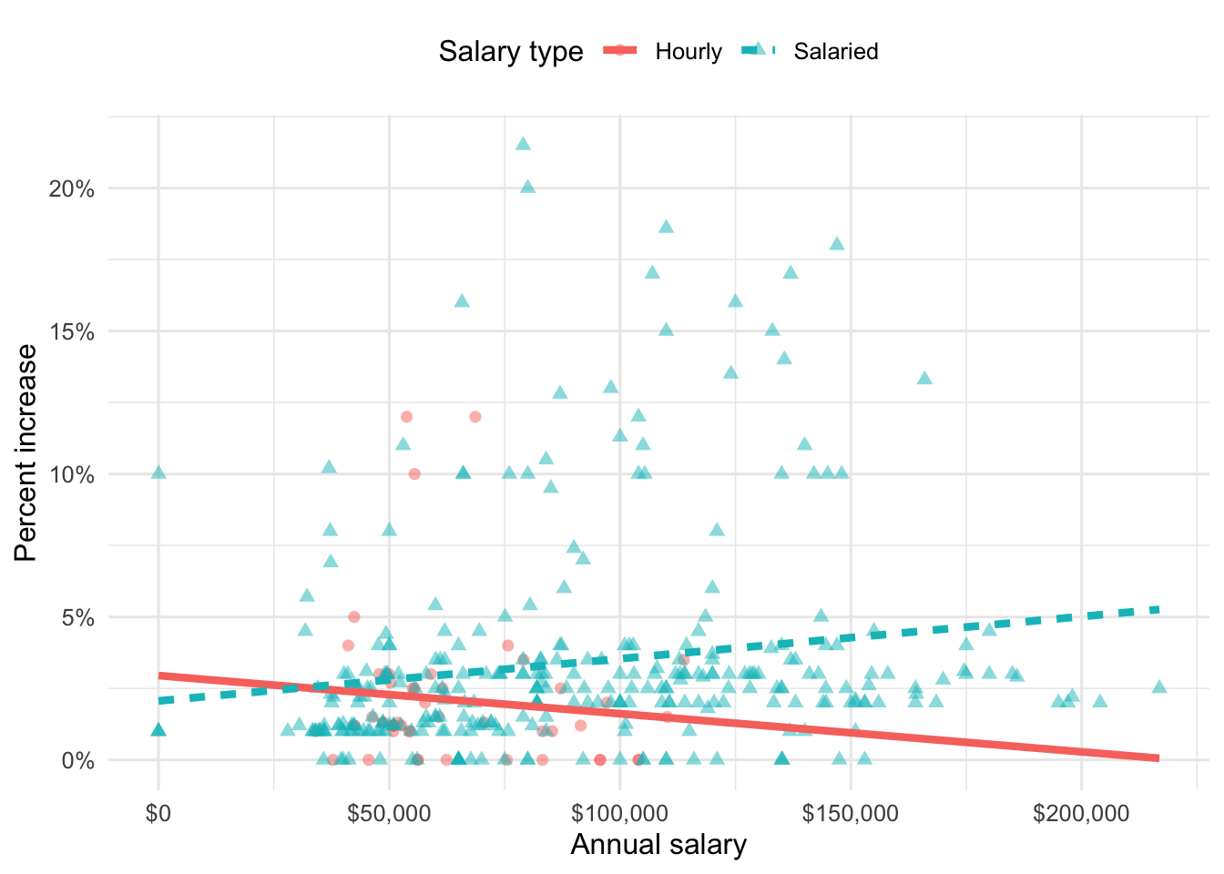
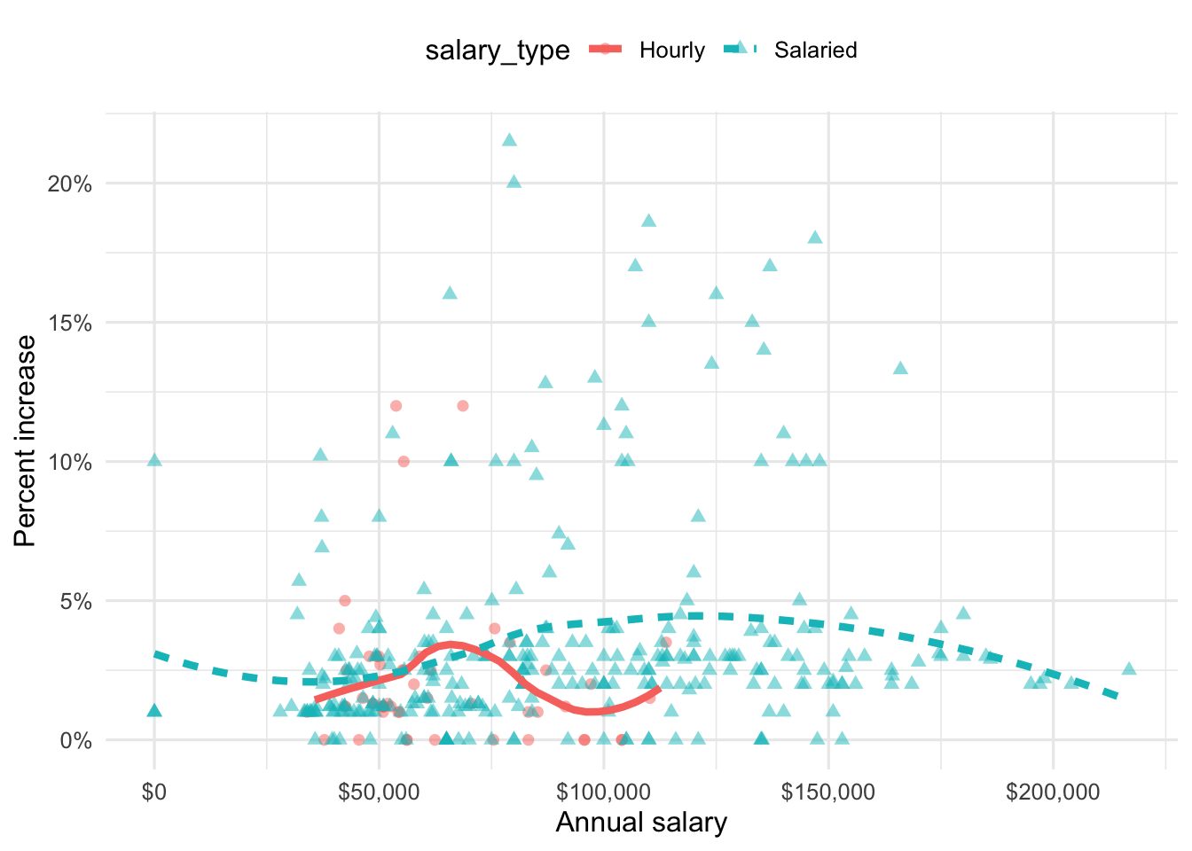
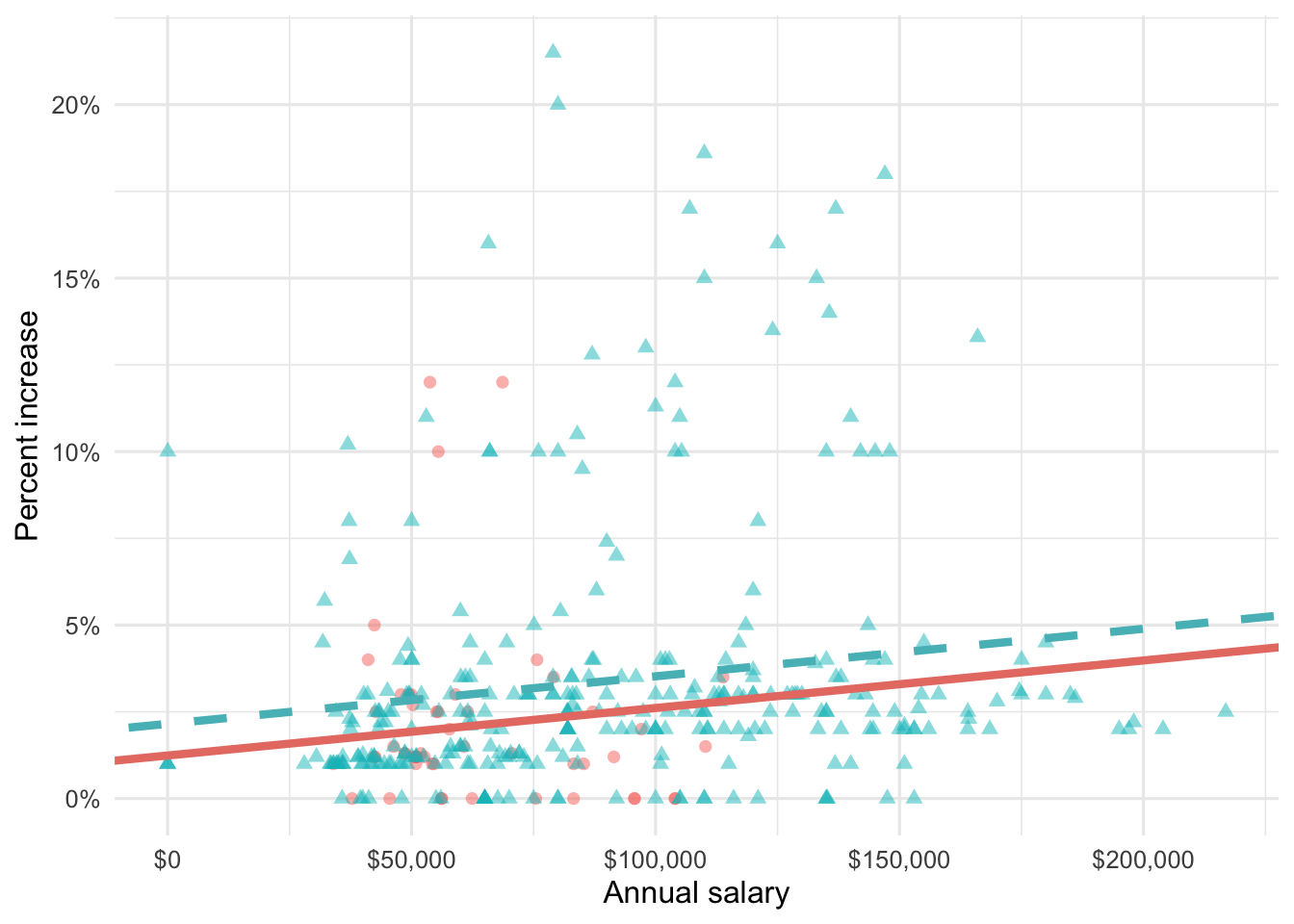
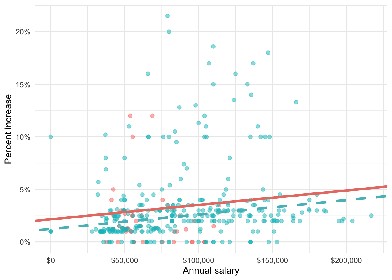
Suppose we fit a model to predict percent_incr from annual_salary and salary_type. A tidy output of the model is shown below.

# A tibble: 3 × 5
  term                 estimate  std.error statistic p.value
  <chr>                   <dbl>      <dbl>     <dbl>   <dbl>
1 (Intercept)         1.24      0.570           2.18 0.0300 
2 annual_salary       0.0000137 0.00000464      2.96 0.00329
3 salary_typeSalaried 0.913     0.544           1.68 0.0938 

Which of the following visualizations represent this model? Explain your reasoning.

(a) Option 1

(b) Option 2

(c) Option 3

(d) Option 4

Figure 1: Visualizations of the relationship between percent increase, annual salary, and salary type

Question 6

Suppose you now fit a model to predict the natural log of percent increase, log(percent_incr), from performance rating. The model is called raise_4_fit.

You’re provided the following:

tidy(raise_4_fit) |>
  select(term, estimate) |>
  mutate(exp_estimate = exp(estimate))

# A tibble: 4 × 3
  term                         estimate exp_estimate
  <chr>                           <dbl>        <dbl>
1 (Intercept)                     -7.15     0.000786
2 performance_ratingSuccessful     6.93  1025.      
3 performance_ratingHigh           8.17  3534.      
4 performance_ratingTop            8.91  7438.      

Based on this, which of the following is true?

a. The model predicts that the percentage increase employees with Successful performance get, on average, is higher by 10.25% compared to the employees with Poor performance rating.

b. The model predicts that the percentage increase employees with Successful performance get, on average, is higher by 6.93% compared to the employees with Poor performance rating.

c. The model predicts that the percentage increase employees with Successful performance get, on average, is higher by a factor of 1025 compared to the employees with Poor performance rating.

d. The model predicts that the percentage increase employees with Successful performance get, on average, is higher by a factor of 6.93 compared to the employees with Poor performance rating.

Part 2 - Movies

The data for this part comes from the Internet Movie Database (IMDB). Specifically, the data are a random sample of movies released between 1980 and 2020.

The name of the data frame used for this analysis is movies, and it contains the variables shown in Table 1.

Table 1: Data dictionary for movies

Variable	Description
name	name of the movie
rating	rating of the movie (R, PG, etc.)
genre	main genre of the movie.
runtime	duration of the movie
year	year of release
release_date	release date (YYYY-MM-DD)
release_country	release country
score	IMDB user rating
votes	number of user votes
director	the director
writer	writer of the movie
star	main actor/actress
country	country of origin
budget	the budget of a movie (some movies don’t have this, so it appears as 0)
gross	revenue of the movie
company	the production company

The first thirty rows of the movies data frame are shown in ?@tbl-data, with variable types suppressed (since we’ll ask about them later).

Part 2a - Score vs. runtime

In this part, we fit a model predicting score from runtime and name it score_runtime_fit.

score_runtime_fit <- linear_reg() |>
  fit(score ~ runtime, data = movies)

Figure 2 visualizes the relationship between score and runtime as well as the linear model for predicting score from runtime. The top three movies in ?@tbl-data are labeled in the visualization as well. Answer all questions in this part based on Figure 2.

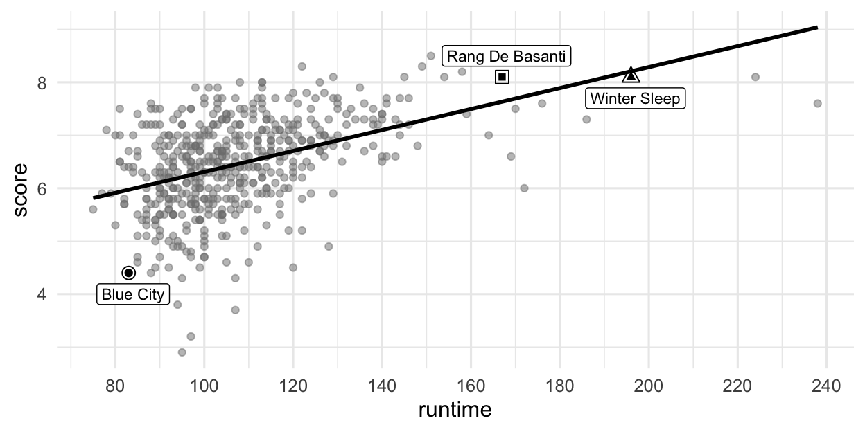
Figure 2: Scatterplot of score vs. runtime for movies.

Question 7

Partial code for producing Figure 2 is given below. Which of the following goes in the blank on Line 2? Select all that apply.

movies |>
  mutate(runtime = ___) |>
  ggplot(aes(x = runtime, y = score)) +
  geom_point(alpha = 0.5) +
  geom_smooth(method = "lm", se = FALSE)
  # additional code for annotating Blue City on the plot

1. grepl(" mins", runtime)

2. grep(" mins", runtime)

3. str_remove(runtime, " mins")

4. as.numeric(str_remove(runtime, " mins"))

5. na.rm(runtime)

Question 8

Based on this model, order the three labeled movies in Figure 2 in decreasing order of the magnitude (absolute value) of their residuals.

1. Winter Sleep> Rang De Basanti > Blue City

2. Winter Sleep> Blue City > Rang De Basanti

3. Rang De Basanti > Winter Sleep> Blue City

4. Blue City > Winter Sleep > Rang De Basanti

5. Blue City > Rang De Basanti > Winter Sleep

Question 9

The R-squared for the model visualized in Figure 2 is 31%. Which of the following is the best interpretation of this value?

1. 31% of the variability in movie runtimes is explained by their scores.

2. 31% of the variability in movie scores is explained by their runtime.

3. The model accurately predicts scores of 31% of the movies in this sample.

4. The model accurately predicts scores of 31% of all movies.

5. The correlation between scores and runtimes of movies is 0.31.

Part 2b - Score vs. runtime or year

The visualizations below show the relationship between score and runtime as well as score and year, respectively. Additionally, the lines of best fit are overlaid on the visualizations.

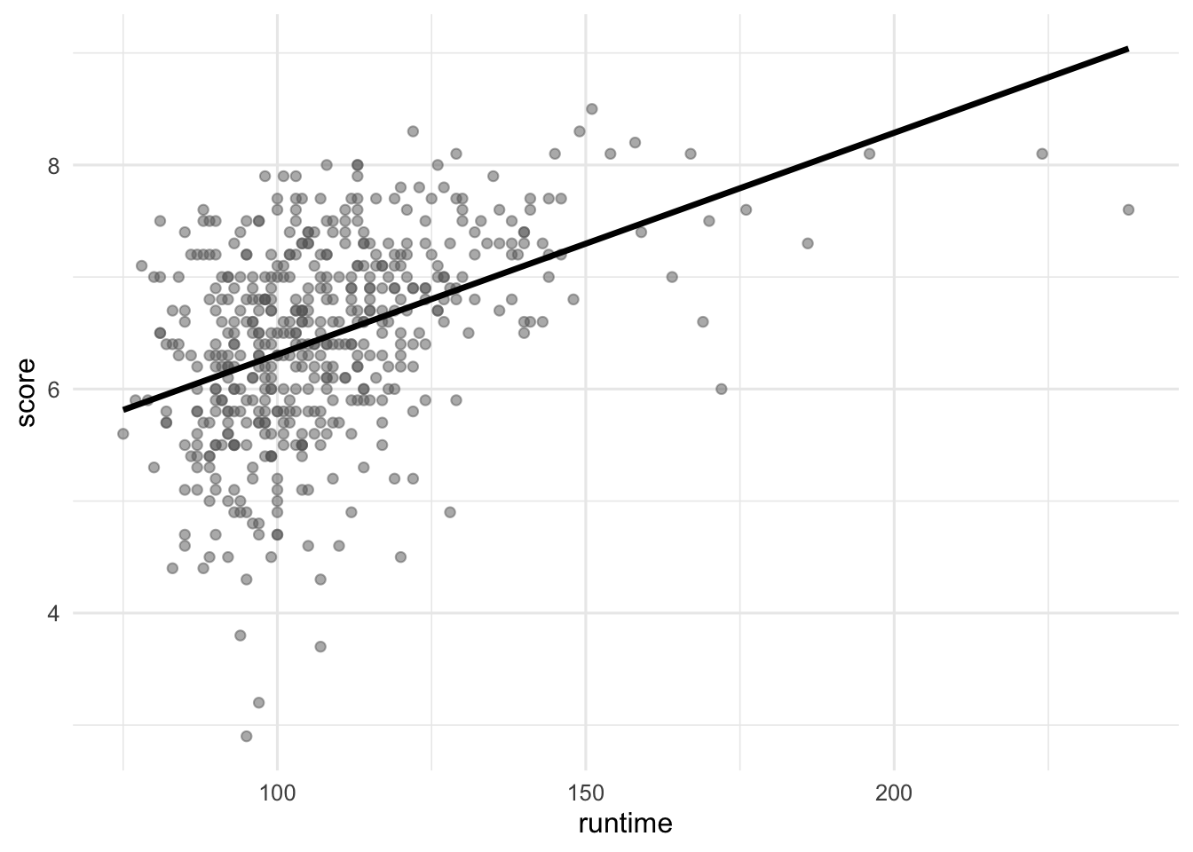
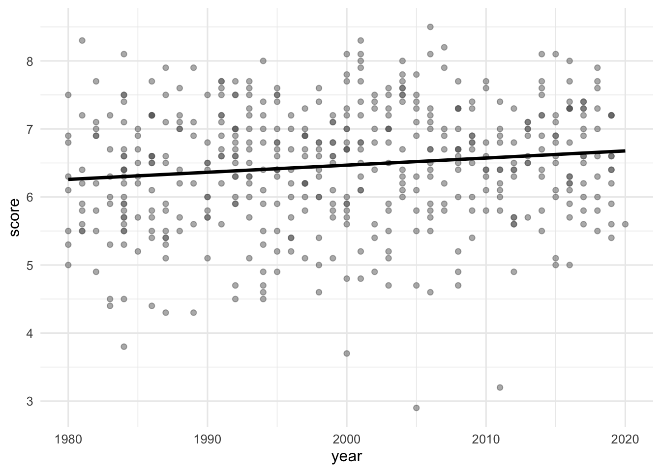
The correlation coefficients of these relationships are calculated below, though some of the code and the output are missing. Answer all questions in this part based on the code and output shown below.

movies |>
  __blank_1__(
    r_score_runtime = cor(runtime, score),
    r_score_year = cor(year, score)
  )

# A tibble: 1 × 2
  r_score_runtime r_score_year
            <dbl>        <dbl>
1           0.434. __blank_2__       

Question 10

Which of the following goes in __blank_1__?

1. summarize

2. mutate

3. group_by

4. arrange

5. filter

Question 11

What can we say about the value that goes in __blank_2__?

1. NA

2. A value between 0 and 0.434.

3. A value between 0.434 and 1.

4. A value between 0 and -0.434.

5. A value between -1 and -0.434.

Part 2c - Score vs. runtime and rating

In this part, we fit a model predicting score from runtime and rating (categorized as G, PG, PG-13, R, NC-17, and Not Rated), and name it score_runtime_rating_fit.

The model output for score_runtime_rating_fit is shown in Table 2. Answer all questions in this part based on Table 2.

Table 2: Regression output for score_runtime_rating_fit.

term	estimate	std.error	statistic	p.value
(Intercept)	4.525	0.332	13.647	0.000
runtime	0.021	0.002	10.702	0.000
ratingPG	-0.189	0.295	-0.642	0.521
ratingPG-13	-0.452	0.292	-1.547	0.123
ratingR	-0.257	0.285	-0.901	0.368
ratingNC-17	-0.355	0.486	-0.730	0.466
ratingNot Rated	-0.282	0.328	-0.860	0.390

Question 12

Which of the following is TRUE about the intercept of score_runtime_rating_fit? Select all that are true.

1. Keeping runtime constant, G-rated movies are predicted to score, on average, 4.525 points.

2. Keeping runtime constant, movies without a rating are predicted to score, on average, 4.525 points.

3. Movies without a rating that are 0 minutes in length are predicted to score, on average, 4.525 points.

4. All else held constant, movies that are 0 minutes in length are predicted to score, on average, 4.525 points.

5. G-rated movies that are 0 minutes in length are predicted to score, on average, 4.525 points.

Question 13

Which of the following is the best interpretation of the slope of runtime in score_runtime_rating_fit?

1. All else held constant, as runtime increases by 1 minute, the score of the movie increases by 0.021 points.

2. For G-rated movies, all else held constant, as runtime increases by 1 minute, the score of the movie increases by 0.021 points.

3. All else held constant, for each additional minute of runtime, movie scores will be higher by 0.021 points on average.

4. G-rated movies that are 0 minutes in length are predicted to score 0.021 points on average.

5. For each higher level of rating, the movie scores go up by 0.021 points on average.

Question 14

Fill in the blank:

R-squared for score_runtime_rating_fit (the model predicting score from runtime and rating) _________ the R-squared the model score_runtime_fit (for predicting score from runtime alone).

1. is less than

2. is equal to

3. is greater than

4. cannot be compared (based on the information provided) to

5. is both greater than and less than

Question 15

The model score_runtime_rating_fit (the model predicting score from runtime and rating) can be visualized as parallel lines for each level of rating. Which of the following is the equation of the line for R-rated movies?

1. \(\widehat{score} = (4.525 - 0.257) + 0.021 \times runtime\)

2. \(score = (4.525 - 0.257) + 0.021 \times runtime\)

3. \(\widehat{score} = 4.525 + (0.021 - 0.257) \times runtime\)

4. \(score = 4.525 + (0.021 - 0.257) \times runtime\)

5. \(\widehat{score} = (4.525 + 0.021) - 0.257 \times runtime\)

Part 3 - Miscellaneous

Question 16

Which of the following is the definition of a regression model? Select all that apply.

a. \(\hat{y} = b_0 + b_1 X_1\)

b. \(y = \beta_0 + \beta_1 X_1\)

c. \(\hat{y} = \beta_0 + \beta_1 X_1 + \epsilon\)

d. \(y = \beta_0 + \beta_1 X_1 + \epsilon\)

Question 17

Choose the best answer.

A survey based on a random sample of 2,045 American teenagers found that a 95% confidence interval for the mean number of texts sent per month was (1450, 1550). A valid interpretation of this interval is

1. 95% of all teens who text send between 1450 and 1550 text messages per month.
2. If a new survey with the same sample size were to be taken, there is a 95% chance that the mean number of texts in the sample would be between 1450 and 1550.
3. We are 95% confident that the mean number of texts per month of all American teens is between 1450 and 1550.
4. We are 95% confident that, were we to repeat this survey, the mean number of texts per month of those taking part in the survey would be between 1450 and 1550.

Question 18

Define the term “parsimonious model”.

Part 4 - Building a spam filter

The data come from incoming emails in David Diez’s (one of the authors of OpenIntro textbooks) Gmail account for the first three months of 2012. All personally identifiable information has been removed. The dataset is called email and it’s in the openintro package.

The outcome variable is spam, which takes the value 1 if the email is spam, 0 otherwise.

Question 19

1. What type of variable is spam? What percent of the emails are spam?

2. What type of variable is dollar - number of times a dollar sign or the word “dollar” appeared in the email? Visualize and describe its distribution, supporting your description with the appropriate summary statistics.

3. Fit a logistic regression model predicting spam from dollar. Then, display the tidy output of the model.

4. Using this model and the predict() function, predict the probability the email is spam if it contains 5 dollar signs. Based on this probability, how does the model classify this email?

   Note

   To obtain the predicted probability, you can set the type argument in predict() to "prob".

Question 20

1. Fit another logistic regression model predicting spam from dollar, winner (indicating whether “winner” appeared in the email), and urgent_subj (whether the word “urgent” is in the subject of the email). Then, display the tidy output of the model.

2. Using this model and the augment() function, classify each email in the email dataset as spam or not spam. Store the resulting data frame with an appropriate name and display the data frame as well.

3. Using your data frame from the previous part, determine, in a single pipeline, and using count(), the numbers of emails:

   • that are labelled as spam that are actually spam
   • that are not labelled as spam that are actually spam
   • that are labelled as spam that are actually not spam
   • that are not labelled as spam that are actually not spam

   Store the resulting data frame with an appropriate name and display the data frame as well.

4. In a single pipeline, and using mutate(), calculate the false positive and false negative rates. In addition to these numbers showing in your R output, you must write a sentence that explicitly states and identified the two rates.

Question 21

1. Fit another logistic regression model predicting spam from dollar and another variable you think would be a good predictor. Provide a 1-sentence justification for why you chose this variable. Display the tidy output of the model.

2. Using this model and the augment() function, classify each email in the email dataset as spam or not spam. Store the resulting data frame with an appropriate name and display the data frame as well.

3. Using your data frame from the previous part, determine, in a single pipeline, and using count(), the numbers of emails:

   • that are labelled as spam that are actually spam
   • that are not labelled as spam that are actually spam
   • that are labelled as spam that are actually not spam
   • that are not labelled as spam that are actually not spam

   Store the resulting data frame with an appropriate name and display the data frame as well.

4. In a single pipeline, and using mutate(), calculate the false positive and false negative rates. In addition to these numbers showing in your R output, you must write a sentence that explicitly states and identified the two rates.

5. Based on the false positive and false negatives rates of this model, comment, in 1-2 sentences, on which model (one from Question 20 or Question 21) is preferable and why.